PowerBI.tips

Month: February 2018

Power BI Connections: Live Connection
Of all the connection types, I’ve always gravitated towards this one. I imagine it is because I come from the database developer side of things. I’m a big fan of doing things one time, and having one version that controls many reports is extremely appealing. In fact, this topic was my first blog on Power BI so long ago (here for those feeling nostalgic). The live connection is the most powerful of all the connections that Power BI has to offer in my opinion.

Before we dive into the deep stuff, are you aware that you can use this connection type without your own instance of Analysis Services? Let me explain. Anyone who uses the “Power BI Service” connector that was first made available in April 2017 and released to GA in August 2017 is using a live connection to an Analysis Services Instance hosted in in your Power BI tenant. In fact, each time you build a Power BI report in the Desktop, you are building a Tabular model that is then created in the cloud upon publish! This live connection method allows you to gain a bit more control. You can deploy a single dataset to the Service and re-use it to build multiple reports! Having your own instance of Analysis Services on premises or Azure lets you maximize your development and deployment efforts and truly create a sustainable reporting solution.

The evolution of a Power BI solution “should” typically land in a space where a centralized or several centralized models are being used as the backbone for the vast majority of Power BI reports. This centralized approach is imperative in order for large scale BI initiatives to be successful. SQL Server Analysis Services Tabular is the typical implementation that I see most often employed due to the relational nature, compression, in memory storage and speed. That being said, lets dive into the details of what a centralized model gives us, and the pros & cons of the Power BI Live Connection.

Cons:
- Most limiting of all in terms of disabling Power BI features.
Desktop Live Connection

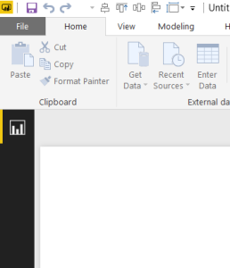
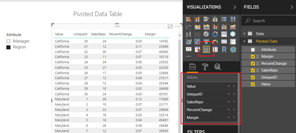
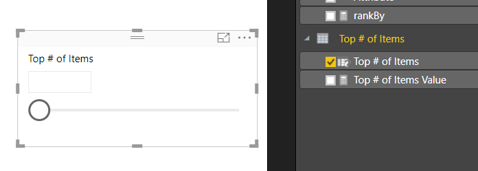
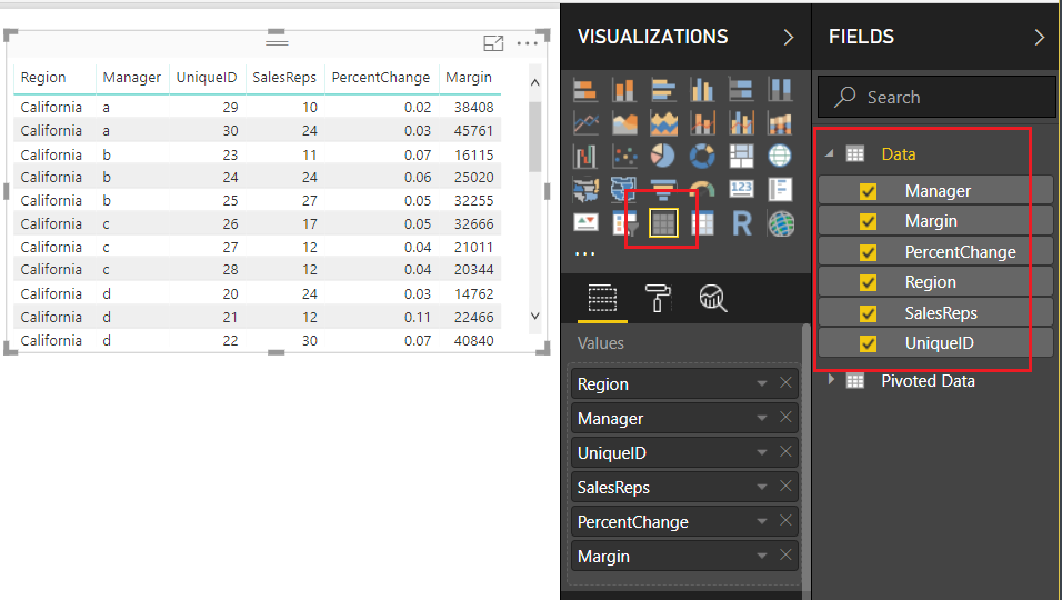
Notice: the Data and Relationships icons are not visible after making a Live Connection.

This is without a doubt the most intimidating to the end user that isn’t familiar with the live connection. As with Direct Query, there are features and capabilities in the Power BI Desktop that are just flat out turned off or completely gone. ETL / M / Query Editor? Gone. Data pane, DAX tables, Calculated columns? Gone. Power BI has become only the front end of the process. The expectation is that you are doing all the data mashup / ETL and modeling behind the scenes and as such, these features are all removed.

However, a really great addition in the May 2017 Desktop release was the addition of allowing measures to be created on top of the live connection. This means that if you have a couple measures you need to add to a single report, you can easily add those in the Power BI Desktop without the need to have them added to the model.
- Cost
Without a doubt one of the most appealing aspects of Power BI is the price. It is amazing the amount of power and value you get for $10/month. (Desktop is free, but let’s just call it $10 because you need a Pro license to share). When you scale up and start to use enterprise level tools you need to look at the costs that those include. This post won’t go into details because there is a myriad of options out there and the number of options increase exponentially when you start comparing Azure to on-premises. Suffice to say, you’re looking at a much heftier investment regardless.
- Different Tools
Another drawback to this connection is that we are now pulled out of the Desktop as a standalone solution and thrown into development areas. At bare minimum we’ll most likely be using Visual Studio, Team Foundation Server for version control, possibly SSIS, SQL Databases and SSAS. Throw in Azure and you might be using Azure SQL Data Warehouse with Azure Data Factory and Azure Analysis Services…

Pros:
- Change Control
This feature that can be implemented by Team Foundation Services allows for a developer to manage their code. In the context of the model, this means that I can check in/check out and historically track all the changes to the model. Which in turn allows me to roll back to a previous version, control who has access to the model and secure the access to the model to a known group.
- Central model that supports many reports
Hands down the benefit to the model / live connection is that I can build a central model that supports a vast number of reports. This streamlines development, lowers the time to implement changes across all reports from IT and centralizes calculations so that all parties are using the same metrics.
- No memory or size constraints in Power BI
Another great feature is that a dedicated server / Azure implementation has the capability to scale up to whatever RAM is necessary to support the model. The limitations of the Desktop are gone, and Power BI capable of handling insanely high volumes of data. This is because the heavy lifting is happening behind the scenes. A prime example of this the new MSFT demonstration that uses 10 billion rows of data related to NY taxis. (Did you catch that? That is a “B” for “BILLION”) I saw it for the first time at PASS Summit 2017, but you can see a quick demo of that below, or here in the first portion of this scale up & diagnostic video.

Now, the underlying hardware in Azure must be immense for this to contain the 9TB of data, but I still think it is amazing that Power BI can provide the same drag and drop experience with quick interaction on a dataset that large. Simply amazing.
- More Secure & Better security
Along with the security of being permissioned to access the model there is an extremely valid argument related to security that just make a SSAS model better. The argument is that while the functionality exists in the Power BI Desktop to enable row level security, the vast majority of the time, the report author shouldn’t control access to certain sensitive information. Having that live in a file accessible by others to be modified isn’t something that passes muster in most orgs. With a model that has limited access, change control and tracking, and process for deployment the idea that a DAX function controlling a security access level to information becomes more palatable.
- Partitions
This feature enters stage left and it is just “Awesome”. Partitions in a model allow you to process, or NOT process, certain parts of the model independently from one another. This gives an immense amount of flexibility in a large-scale solution and make the overall processing more efficient. Using partitions allows you to only process the information that changes and thus reduce the number of resources, reduce processing, and create an efficient model.

All in all, a lot of this article was about model options behind the scenes, but effectively this is the core of the Live Connection. It is all the underlying Enterprise level tools that are required to effectively use the live connection against a SSAS instance. In some respects, I hope that this gives you some understanding of the complexity and toolsets that are actively being used when you are using Power BI in general. All these technologies are coupled together and streamlined to a clean user-friendly tool that provides its users with immense power and flexibility. I hope you enjoyed this series and that it brought some clarity around the different connection types within Power BI.

Thanks for reading! Be sure to follow me on Twitter and LinkedIn to keep up to date with Power BI related content.
February 26, 2018
Crazy Table Gymnastics – Part 2 – Build Support Materials
This is part 2 in the 3 part series on developing super cool tables using some fancy measures. In part 1 we walked through how to build a table that uses an un-pivoted data source in the Query Editor. This technique allows you to change the types of categorical values in a table. If you missed part 1 and want to get caught up follow this link. Now, continuing with the series, Part 2, we will build the supporting materials (Selector Table, What If Slicers, and measures) for the report.

Once we are done the final product will look like the following:

<span data-mce-type="bookmark" style="display: inline-block; width: 0px; overflow: hidden; line-height: 0;" class="mce_SELRES_start"></span>

Part 2… Go.

To make sure we are starting off on the correct step. We left off part 1 when we had completed a Pivoted Data Table and included an Attribute Slicer that would allow us to toggle between the Manager and Region Categories. Your table should look like the following diagram: (If you don’t have this you might want to start with Part 1 found here)

Pivoted Data Table

Note: I have also included a Slicer which is used with the Attribute field.

Next, we will need to add a table that will allow us to use the SalesReps, PercentChange, and Margin column headers in our report. On the Home ribbon click Edit Queries, then select New Source on the Home ribbon. In the Get Data window select Blank Query, click Connect to proceed. Open the advanced editor by clicking the Advanced Editor button found on the Home ribbon. Enter the following M code into the Advanced Editor:
```
let
   Source = #"Pivoted Data",
   #"Kept First Rows" = Table.FirstN(Source,1),
   #"Removed Columns" = Table.RemoveColumns(#"Kept First Rows",{"Attribute", "Value", "UniqueID"}),
   #"Unpivoted Columns" = Table.UnpivotOtherColumns(#"Removed Columns", {}, "Attribute", "Value"),
   #"Removed Columns1" = Table.RemoveColumns(#"Unpivoted Columns",{"Value"})
in
   #"Removed Columns1"
```
Click Done to close the Advanced Editor. Rename the table to Selector. When you are finished your table should look like the following:

Create Selector Table

Click Close & Apply on the Home ribbon to close the Query Editor. Add a slicer with the following selections:

Add Selector Attribute Slicer

Now, we want to detect which of the Attributes have been selected from this table. We can accomplish this by creating a measure using the DAX function SELECTEDVALUE. Right Click on the table named Selector and from the drop down select New Measure. Enter the following DAX equation:
```
rankBy = SELECTEDVALUE(Selector[Attribute])
```
In addition to the knowledge of which column was selected from the selector table, we will also want to detect to make sure at least one categorical value has been selected. The categorical values we are talking about were generated earlier. The values could be either the Manager or Region values of the Attribute column in the Pivoted Data table. Using the ISFILTERED DAX function enables this section. Add the following measure to the Pivoted Data table:
```
Attribute Filtered = ISFILTERED('Pivoted Data'[Attribute])
```
Next, we need to gather some user input in the form of a number from 1 to 10. To input this information we need to produce a What If Parameter. On the Modeling ribbon click New Parameter in the What If section of the ribbon. Enter the following information into the What-if parameter dialog box:

What If Parameter

Note: Don’t forget to change the Name of the parameter.

Click OK to proceed. Power BI will automatically produce a measure table, a measure and a slicer on the report page.

Slicer Produced by What-if

Note: By default there is nothing selected in the box. However, you can adjust the slicer and a number will appear within the value box. You can also type in a number between 1 and 10 to the box to adjust the value.

This is where we go crazy with DAX. This portion of DAX is where all the magic happens.

We start off by building our totals measures. Place all these measures in the Pivoted Data table.
```
Total % Change = MAX( 'Pivoted Data'[PercentChange] )
Total Margin = SUM( 'Pivoted Data'[Margin] )
Total SalesReps = SUM( 'Pivoted Data'[SalesReps] )
```
These will be used repeatedly in our next group of DAX formulas.

The following measures will produce a calculated ranking for each numerical column. OK, Pause, This part really excites me here because the next few measures are where the magic happens. Pay close attention to what is happening here. Un-Pause, by using the DAX Switch function we can dynamically tell Power BI to adjust which column we want to see ranked by the top items. For example, if we select SalesReps in our attribute slicer. The following measures will automatically rank all the items in the table by the column named SalesReps. Thus, the items with the highest counts of SalesReps will be listed first. When you select Margin, the table will automatically adjust and re-rank the items by the Margin column. This is being done in the switch statement. For each column we are calculating custom rankings and then hiding or replacing values with the Blank() DAX function to not show items we don’t want.

Enter the following three measures into the Pivoted Data Table:
```
Rank Margin = if( [Attribute Filtered],
    SWITCH( [rankBy]
        ,"Margin", CALCULATE( [Total Margin], FILTER('Pivoted Data', RANKX( ALLEXCEPT('Pivoted Data','Pivoted Data'[Value]), [Total Margin]) <= [Top # of Items Value]) )
        ,"PercentChange", CALCULATE( [Total Margin], FILTER('Pivoted Data', RANKX( ALLEXCEPT('Pivoted Data','Pivoted Data'[Value]), [Total % Change]) <= [Top # of Items Value]))
        ,"SalesReps", CALCULATE( [Total Margin], FILTER('Pivoted Data', RANKX( ALLEXCEPT('Pivoted Data','Pivoted Data'[Value]),[Total SalesReps]) <= [Top # of Items Value]))
    )
    , BLANK() )

Rank PercentChange = if( [Attribute Filtered],
     SWITCH( [rankBy],
       "PercentChange", CALCULATE( [Total % Change], FILTER('Pivoted Data', RANKX( ALLEXCEPT('Pivoted Data','Pivoted Data'[Value]), [Total % Change]) <= [Top # of Items Value]))
       ,"Margin", CALCULATE( [Total % Change], FILTER('Pivoted Data', RANKX( ALLEXCEPT('Pivoted Data','Pivoted Data'[Value]), [Total Margin]) <= [Top # of Items Value]))
       ,"SalesReps", CALCULATE( [Total % Change], FILTER('Pivoted Data', RANKX( ALLEXCEPT('Pivoted Data','Pivoted Data'[Value]), [Total SalesReps]) <= [Top # of Items Value]))
    )
    , BLANK() )

Rank SalesReps = if( [Attribute Filtered],
    SWITCH( [rankBy]
        ,"SalesReps", CALCULATE( [Total SalesReps], FILTER('Pivoted Data', RANKX( ALLEXCEPT('Pivoted Data','Pivoted Data'[Value]), [Total SalesReps]) <= [Top # of Items Value]))
        ,"Margin", CALCULATE( [Total SalesReps], FILTER('Pivoted Data', RANKX( ALLEXCEPT('Pivoted Data','Pivoted Data'[Value]), [Total Margin]) <= [Top # of Items Value]))
        ,"PercentChange", CALCULATE( [Total SalesReps], FILTER('Pivoted Data', RANKX( ALLEXCEPT('Pivoted Data','Pivoted Data'[Value]), [Total % Change]) <= [Top # of Items Value]))
    )
    , BLANK() )
```
Whew, that was a ton of measures. All the key components are complete now. In part 3 we will clean up our report page and make it shine. I hope you enjoyed this tutorial. Also, follow me on Twitter and Linkedin where I will post all the announcements for new tutorials and content.
February 21, 2018
Crazy Table Gymnastics – Part 1 – Dynamic Column Categories
When I teach Power BI to new users, there are typically questions about how to get Power BI to act more like Pivot Tables in Excel. Through my discussions, two key pieces of functionality stand out to me that people want.
1. They would like to select a categorical property to adjust the table. In this scenario a user would want to select the State, Sales Territory, or something else that describes a breakdown of the data. This is similar to adding a field of data into the Rows selection for Pivot Tables.
2. They want the ability to rank a column and select only the top N number of items in a given column. Imagine that you have Sales Units, Revenue, or some other numerical column. Then based on a selected column such as Sales Units, I want to see the top 3 or 4 sales items. This would be a similar in the excel experience when you modify the filters for a given pivot table column.
Disclaimer: This is quite a large topic and therefore I have broken this up into three segments for read-ability. Thus, to poke your curiosity below is the final example of the report. We will walk through reach phase of this report, so you can produce this dynamic table.

<span data-mce-type="bookmark" style="display: inline-block; width: 0px; overflow: hidden; line-height: 0;" class="mce_SELRES_start"></span>

This series of blogs will be broken up into three parts.

Part 1: Build a Table or Matrix visual that can dynamically change based on a slicer

Part 2: Build supporting tables & measures

Part 3: Bring it all together for the final report

OK, hold on tight, here we go!

Let’s begin with acquiring our data. Open Power BI Desktop. Click Get Data on the Home ribbon and select Excel. When the Open dialog box opens enter the following file name, and click Open:

https://powerbitips.blob.core.windows.net/powerbitipsdatas/SampleData.xlsx

The Navigator window will open showing you the contents of the file. Select the Data Table by clicking in the square next to the word labeled Data, click Edit to load the data and enter the Query Editor.

Load Data from Excel

Next, Right Click on the table labeled Data in the Queries pane, from the drop-down menu select Reference.

Create Reference Query

This will produce a second table labeled Data (2). In the Properties pane on the right side of the screen edit the name of the query to Pivoted Data. Select the columns UniqueID, SalesReps, Margin, and PercentChange by holding Ctrl and clicking on each column. While keeping all four (4) columns selected right click on the last column and select Unpivot Other Columns.

Unpivot Columns

Note: It is important to notice that we selected Unpivot Other Columns instead of selecting the Region and Manager columns and selected Unpivot Columns. Selecting Region and Manager and selecting Unpivot Columns will achieve the same results, but if our excel file or underlying data set adds more Categorical columns our query will break. Using this technique creates a flexible query that can handle any number of new categorical columns. You know your data the best, and how it will change over time. It is important to consider these aspects when loading data via the Query Editor.

We have completed our data load. On the Home ribbon click Close & Apply to complete the data load for our two tables, Data and Pivoted Data.

Load the Fields from the Data table into a Table Visual, as shown below:

Data Fields Loaded Into Table

For the following fields SalesReps, PercentChange, and Margin change the Fields to SUM by clicking on the Triangle next to each field’s name. We will use this information to confirm that our Pivoted table is providing the correct data.

Change Fields to Sum

Add a second Table visual and bring over the fields from the second data set, our Pivoted Data table. Be sure to leave off the Attribute column as this will not be needed in this second table.

Table for Pivoted Data

Add a Slicer to the report layout and add the column labeled Attribute from the Pivoted Data table.

Add Slicer

Notice we now have the ability to select either the Manager Column or the Region column. By doing so, we are able to change the columns within our table to only show the items relevant to our slicer selection. Pretty cool.

Using The Slicer

It’s also important to note here that in our Pivoted Data Table, we can only acquire the correct totals with a single attribute selected. When the slicer has no selection our totals for SalesReps, PercentChange and Margin are all twice the amount they should be. Later on, in part 2 of this tutorial, we will fix this using measures.

Data In Both Tables Match

Thanks for reading along. Stay tuned for part 2 where we will build supporting data tables to aid the user experience on the report page. If you like what you learned, please forward this on to someone else who would enjoy these free tutorials. Also, follow me on Twitter and Linkedin where I will post all the announcements for new tutorials and content.
February 14, 2018