Tag: Beginner

  • Query Settings – Fixing a Missing File

    Query Settings – Fixing a Missing File

    One of the most important concepts to learn within Power BI Desktop is how to build a Data Model.

    Note: In simple terms the Data Model is data that is collected from the get data function.  In your data model you can build multiple queries.  This data is stored in the file.  The data storage is very efficient as the data compressed down to approximately a 4:1 ratio.  1000 KB file will compact down to approximately 250 KB when loaded into Power BI.  From my current understanding all data is loaded into the memory of the computer.  Thus, if you are having performance issues it could be in part due to the RAM of your computer.  

    As you begin to craft more data models you will learn little tips and tricks along the way to make an efficient Data Model for your visualizations.  I have found that the most challenging part of building the data model is structuring the data in a way that will make your selected visual make sense.  This may mean you need to add a measure or a calculated column or a ranking to a data set. Alright lets get started.

    Here are the Resources for this tutorial:

    • Power BI Desktop (I’m using the March 2016 version, 2.33.4337.281) download the latest version from Microsoft Here.
    • We are going to work through the Power BI Desktop file that we built in the Loading Excel Files Into Power BI Tutorial.  You can follow the link to create the Power BI Desktop (pbix) file in the tutorial.  For convenience, the completed file can be downloaded here: Import Excel Tutorial.

    I’m going to start off by extracting the Import Excel Tutorial.zip file to my desktop.  Once the file has been extracted we can open the containing folder.  In this folder there are two files the source data in the excel file and the Power BI Desktop file.

    Note: A Power BI Desktop file has a .pbix file format ending.

    Open the Import Excel.pbix file.  First click the Home ribbon and then click the Refresh button.  Most likely there will be an error similar to the following message.
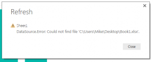
    Can't find file
    Message box when file can’t be found

    This type of message occurs when you refresh a query and the file is missing or can’t be found.  This is because when i originally built the Power BI Desktop tutorial the excel file that is supply the information was located on my desktop.  This is a common problem when you build connections to local files stored on your computer.  If you move a file into a different folder then the connection will break.

    To resolve this close the message window by clicking Close. on the Home ribbon click the Edit Queries button.  The Query Editor window will be presented.  In a large yellow bar in the data view portion of the window (circled in red) is the error message.

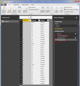
    Note: Circled in blue is the Query Settings window.  This window is the window for all the applied steps to transform the data.  You can change the name of the query in the name box.  From the view we have selected we can see that the step entitled Changed Type is currently selected (seen circled in blue).

    Click the grey button labeled Go To Error which is found in the yellow error box.
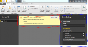
    Go To Error
    Error seen inside Query Editor

    Upon clicking the Go To Error button the selection in the Query Settings button to the Source Step.  This is where the query has failed.  More information about the failure is shown in another yellow error box.  This time click Edit Settings in the error box.

    Edit Settings
    Edit Settings in Error window

    Now we have the Load Excel file window prompt open.  In this window Click Browse, navigate to where you extracted all the files downloaded earlier in the tutorial and select the excel document entitled Book1.  Click Open and the new file location will be loaded into the Load Excl Window.  Click OK to complete the settings change.
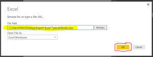
    New File Location
    New File Location

    Now the data is correctly loaded into the data model.  Notice we are still on the step called Source.  Take some time to click through each step, Source – Navigation – Promoted Headers – Changed Type.  As you click on each step you can see how the data is transforming.

    To see the code that is being used to make each step click the View ribbon and check the little box entitled Formula Bar.  This will make a formula bar appear.  When you click on a step the formula bar will reveal the code needed to complete the selected step.
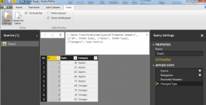
    Toggle the Formula Bar
    Toggling on the Formula Bar

    We can now see the equation, which is similar to how you would write an equation in excel.  The code in the Changed Type step is here:

    = Table.TransformColumnTypes(#"Promoted Headers",{{"ID", Int64.Type}, {"Sales", Int64.Type}, {"Category", type text}})

    The equation is using the M language to transform the data.  More information on the usage of the M language can be found here.

    Note: Couple of pointers about the data shown in the formula.  The function is called Table.TranformColumnTypes.  The source of the data is a variable called #”Promoted Headers”.  The pound sign and the words following in quotations is how the M language passes variables that have a space contained in the language.  Since the prior step has the name “Promoted (space) Headers” the program has to add the pound sign and the quotation marks.  If there is no space in the naming convention such as “PromotedHeaders” then only the PromotedHeaders would be seen in the code and the pound sign and quotes will be gone. See modify coded when I remove the space from the Promoted Headers applied step.

    = Table.TransformColumnTypes(PromotedHeaders,{{"ID", Int64.Type}, {"Sales", Int64.Type}, {"Category", type text}})

    Notice the the pound sign and quotations are missing.

    The second part of the formula is an array which has been written out in curly brackets:

    {
    {"ID", Int64.Type}, 
    {"Sales", Int64.Type}, 
    {"Category", type text}
    }

    I changed the code by adding line returns to make it easier to read.  The coded array has beginning bracket and an ending bracket.  Each parameter is contained in it’s own curly brackets and separated with a comma.  The array is a 2 x 3 array, it has 3 rows and two data points on each row, just like a matrix.  The first data point is the column name.  In the first row the column that is being address is called ID.  The data transformation parameter is called Int64.Type.  This means that the data is an integer type 64 bit.  This repeats for each row until all parameters have been addressed.

    So there you go, we have opened up a query repaired it and learned a little about the formula bar.

    As a side note, as you build queries each button press that you make on the various ribbons in the Query Editor will make a minimum of one step the in the Query Editor.

    Hope you enjoyed this short tutorial about the Query Editor.  Make sure you share below if you liked it.

  • Folder of Files Loaded to Power BI Desktop

    Folder of Files Loaded to Power BI Desktop

    Ok, I’ve got to be honest the first two tutorials (Loading Excel Files, Loading CSV Files) were only there to get things kicked off. Now we are getting to some of the good stuff.

    When I first saw this feature in Power Query for excel I nearly had a conniption.  My first thought is this is going to CHANGE EVERYTHING, and to be perfectly honest it has. My entire view of Excel and Power BI has been shaped by this simple but powerful idea; Automated Data Loading.

    In all my years as an engineer I would have to constantly copy and paste data from one excel file to another. Then perform some transformations just to produce a bar chart or a line graph, uggh.  This is slow and boring.  I was really good at being boring, and I felt like I was able to become quite ingenious by writing macros and automating parts of my data transformations.  Now I have seen the light,  The simple ability of being able to load a group files from a folder is AWESOME!  Had I had this feature in my engineering days I could have saved so much time.  So in true homage of my engineering roots this post is for you, the all mighty data hungry engineer.

    Alright, enough of be babbling, Lets get to it.

    Materials for this Tutorial:

    • Zip file with (3) three excel files download Data Set.
    • Power BI Desktop (I’m using the March 2016 version, 2.33.4337.281) download the latest version from Microsoft Here.

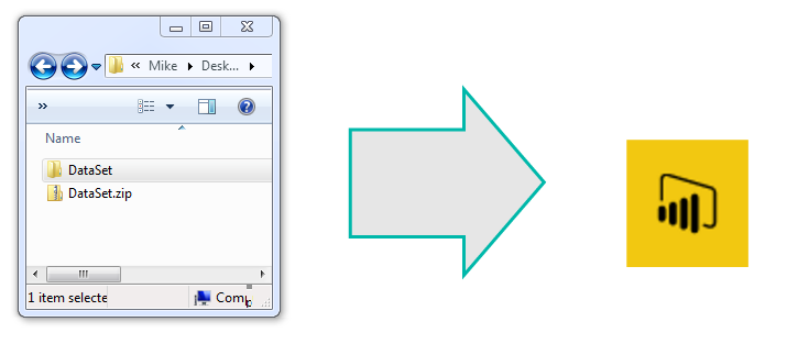
    Lets start off by downloading the Data Set and unzipping the file to a folder called DataSet.  For this demo I unzipped the files to my desktop folder.

    UnZipped Files
    Location for UnZipped Excel Files

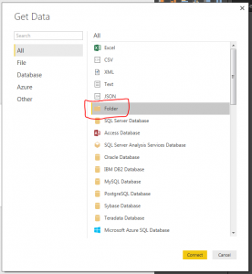
    Next we will open up Power BI Desktop.  On the Home ribbon select the Get Data button.  The Get Data window will be presented and this time we will select the Folder icon in the menu.

    Get Data Folder
    Get Data Folder Icon Selection

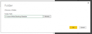
    Click the Connect button at the bottom right of the screen.  A folder window will display.  This is where we will select the location of our data in the folder we unzipped earlier.  Click OK once you’ve selected the location of the folder.

    Folder Path
    Folder Path Location

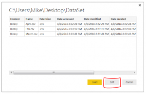
    The next window to open shows the files that Power BI Desktop is able to see in the folder location.  Normally we would press Load and move forward but in this case we want to further manipulate our query to load the data.  Therefore, Click the Edit button to modify the query to load data.

    Folder Location
    View of Files in Selected Folder

    We are now in the Query Editor.  This is where we can manipulate the incoming data before we visualize it.

    Note:  The Query Editor is a graphical representation of the M-language which is used to load data.  Each button press in the Query Editor performs a transformation to your data.  Each step writes a little line of code that handles the transformations.  To see the code Click the View ribbon then click the button labeled Advance Editor.  For more documentation on the M language look at the Microsoft documentation located here.

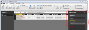
    Here is an image of the files we loaded in from our folder location in the Query Editor.

    Query Editor
    View of Query Editor

    The next step is to combine all the files into one combined data model.  To do this click the Double Down Arrows that are circled in red on the left side in the column called content.  

    Note: I also circled the Query Settings in Red on the right.  The Query Settings window will become very useful, especially when trouble shooting a query.  You will notice as we make additional data transformations more steps will accumulate in the query settings.

    We now have a final view of all the data from each of the three CSV files.

    Data Model
    Loaded Files into the Data model

    The file needs a little clean up to remove some unwanted data rows.  Notice now that we have loaded all three files.  In each file we had a header row.  Now in our data model we have three rows with headers.  We want to use the first row as column names.  To do this, Click the Use First Row as Headers button on the Home ribbon.

    Header Row
    Use First Row as Headers

    Also, notice there are rows of data that contain the initial header rows from the other two files.

    Other Headers
    Header Rows from Other Two Files

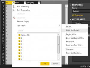
    Now we will apply a filter to remove these rows.  Click the Arrow in the ID row.  This will present a menu.  There are various transformations on this screen, you can sort a row in Ascending, or Descending order, Filter out text items, etc…

    Filter ID Row
    Filter for ID Row

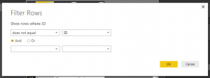
    Click Text Filters and select Does Not Equal and enter ID into the filter.  Click OK to proceed. This will add a step to remove any row that had ID listed in the ID column.

    Filter Rows
    Filter out the Text “ID” from column

    We have transformed our data and now have cleaned the data and it’s ready for use.  Click Close and Apply to load the data to the data model.  Now the data is ready for visualizations.  Thanks for following along.

    Make sure you take some time to share if you enjoyed this tutorial.

  • Import CSV file to Power BI

    Import CSV file to Power BI

    This post is going to be similar to my previous post about Getting Data.  I figure we better cover some of the basics before going crazy with deeper topics.

    Materials for this tutorial:

    • CSV file with some random data, linked here: SampleData in CSV format
    • Power BI Desktop (I’m using the March 2016 version, 2.33.4337.281)

    After I read the previous version I thought it would be helpful to put the materials up at the top and what version I was using.  If you didn’t know Microsoft has been very active in the development of PowerBI.com and Power BI Desktop.  Right now there are weekly updates to PowerBI.com and monthly updates to Power BI Desktop.

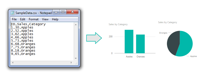
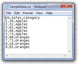
    Starting off like before here is a sample of the data from the csv file.  I’m showing the data in notepad to prove it is a comma separated value file (hence the CSV name).

    csvfile
    CSV File opened in Note Pad

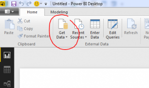
    Alright, lets go get some data.  Open up Power BI Desktop.  Click on the Home ribbon.  Select the Get Data icon.

    Get Data Button
    Button for Get Data

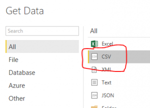
    Now the Get Data window will open.  Next, select the second item labeled CSV from the top of the list on the right.

    Get CSV selection
    CSV selection in the Get Data screen

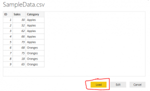
    Click the Connect button at the bottom right hand of the Get Data screen to proceed to the next screen.  Now the open window will let you navigate to the CSV file you would like to import.  Click the Open button at the right of Open window to load the CSV file.  Finally you’ll be presented with the data view of the contents contained inside your CSV file.

    View Of CSV Data
    View of CSV Data file

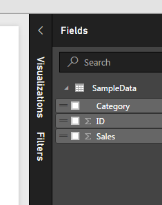
    Once loaded we now have our view of all the columns of data in the Fields viewing pane on the right.  From here we can build our visuals.

    Loaded CSV Columns
    Loaded Columns from CSV file load

    Now, lets throw together a quick visual of the data.

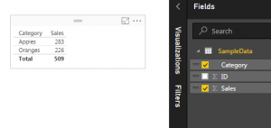
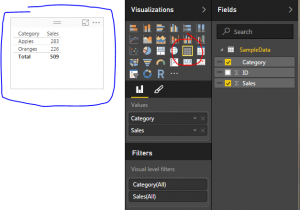
    Start by clicking the check box next to the label titled Category and then click the box next to the label titled Sales.  This will automatically populate a table with the categories in the first column and the sales for each category in the second column.

    Table Visual
    Table of Data

    To open up the Visualizations bar click on the word Visualizations.  This will present all the information relating to the visuals. Upon opening up the visualizations pane there is a small yellow square showing you which visual is selected.

    Selected Visual
    Showing the Selected Visual

    Note: The blue pen highlighting shows the selected visual on the page.  As you build more complex visuals there will be multiple visualizations on your page.  When you select a specific visual, all the properties in the Visualizations Bar show all the properties for the selected visual.  The Table visual is highlighted by the red highlight circle.

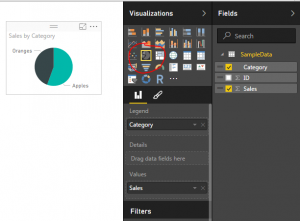
    To change our selected visual to a new visual we will simply select a new icon in the Visualizations bar. Click the icon that looks like a pie chart.

    Pie Chart
    Pie Chart Visualization

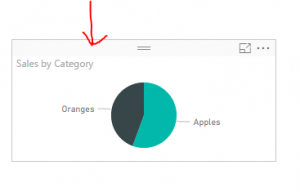
    Cool, but what if I want more awesomeness on my page.  No problem.  Let’s copy our visual.  You can do this by selecting the visual.  To know it is selected look for the slight grey bar at the top of the visual.

    Gray Bar on Visual
    Gray Bar denoting that visual is selected

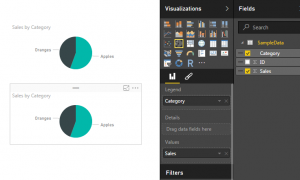
    Copy the visual by using Ctrl + C.  Click any where on the white space on the page.  This will deselect the current visual.  Then paste an identical version of the visual by using Ctrl + V.

    Two Visuals
    Copy and Paste of new Visual

    Ta-da! Now we are really getting somewhere.  Two Amazing visuals, well not quite.  Two identical visuals isn’t very compelling.  Lets change one of the visuals to a different visual.

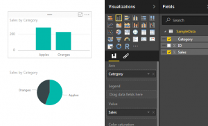
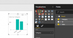
    Select the top visual by clicking on it.  Then select the Stacked Column Chart which is the second icon from the left in the top row.  Selecting this icon will change the visual.

    Bar Chart
    Bar Chart Visual

    And there you have it.  You’ve imported a CSV file and generated two visuals.  Nice job.

    Hope you enjoyed this tutorial.  Leave comments if you have questions or if you want to see something else in a tutorial. If you like what you see please share this post on your selected social network of choice below.

  • Import an Excel file into PowerBI

    Import an Excel file into PowerBI

    We are going to kick this blog off with a simple example of how to load data from excel into Power BI Desktop.

    Note: I’m a firm believer of always understanding your data.  If you are receiving data files or extracts from an automated system or from an individual, trust me it will make a difference.  So, make sure you understand the source of the data and how the structure of your data may change over time.  For example, you have have a column that has both text values and number values; or the data may add additional columns in the future.  Thus, the data load into Power BI Desktop (PBID) will need to be flexible.

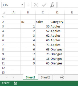
    Lets start off with some simple data in excel:

    Excel Data Image
    Sample of Data in Excel

    We have three columns of data, two have number in it and one has text values.

    For now we will close out of excel and jump over to Power BI Desktop.  Once the program loads we will click the Home ribbon then select the Get Data button.

    Get Data Button
    Button for Get Data

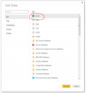
    After pressing the button a new menu will pop up showing us all the sources where data can be ingested from.  The very first item in the list is Excel.  Click the Excel then click the Connect button in the lower right hand corner.

    Excel Data Source
    Select Excel as Data Source

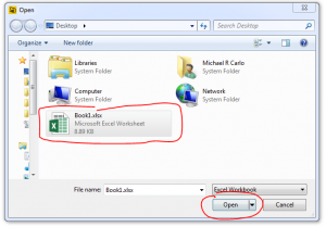
    After clicking Connect a new window will pop up asking for the location of the Excel file.  Navigate to our sample data called Book1.xlsx you can down load the actual file I used here: Book1  I saved my Book1.xlsx file on the desktop of my computer.  Select Book1 and then Click Open.

    Open Excel File
    Open Excel File Dialog Box

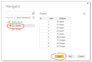
    Next we are presented with the Navigator screen that reveals what is inside the workbook.  There are two sheets.  For now we are only interested in the data on Sheet1.  Select Sheet1 and then click Load.  This will load our data from Sheet1 into the Power BI Desktop data model.

    Navigator Image
    Navigator Selection Screen

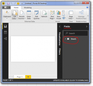
    Now our data has been added to the Power BI Desktop data model.  The data and the various columns we loaded can be found in the tool bar at the far right of PBI called Fields.

    Fields View
    Location of Loaded Excel Data

    Tech Tip: Power BI Desktop (PBI) opening the file and loading the relevant data into the memory of the computer.  This has an approximate 4 to 1 compression ratio.  In practical terms this means that a 100MB file will only consume 25MB of file size in PBI when it is saved.  This is extremely useful as the data model can be quite large when loading multiple data files but the PBI file will compress down to a manageable size.


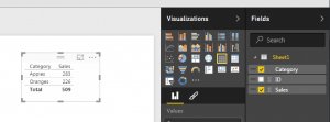
    Make a PBI Table
    Make a Data from Column Sales and Category

    Finally, the Sheet1 data table can be expanded into is respective columns by clicking the triangle next to the table icon.  Finally you can drag and drop the column names into the visualization page to begin making visualizations.  For this demo I used the Category Column and the Sales column to make a table.

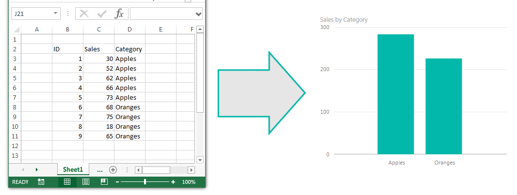
    By selecting a different visualization in the visualizations bar you can change your data table into a Bar Chart.

    Power BI Desktop Bar Chart
    Data Transformed into a Bar Chart

    Well that is it for the first tutorial.  Share your thoughts and comments below.  Let me know if you have any suggestions on what you would like to see next.