Month: December 2017

  • Power BI Connections: Direct Query

    Power BI Connections: Direct Query

    Now that we’ve solidly gotten through the basics in terms of what connection types are in the opening blog, found here, and detailed out what is included in the default connection type of Import found here, let’s get on with some of the more interesting connections.

    Connection Type Outline
    Connection Type Outline

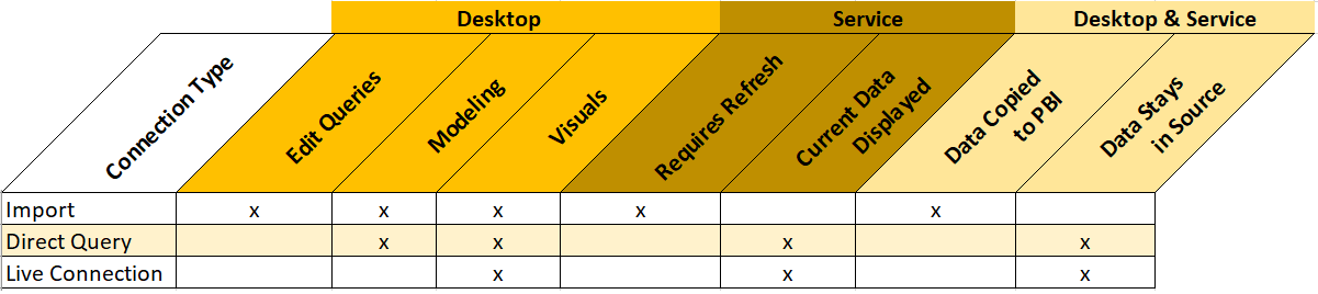
    Direct Query is the first connection type that we will discuss that extends, but at the same time limits functionality in the tool itself. In terms of data access this connection type allows us to access our data in the source system. The supported data sources for direct query can be found here. This is distinctly different than what we observed in the import method.  When using Import, the data is a snapshot and refreshed on a periodic basis, but with Direct Query it is live. “Live” means that with Direct Query the data stays in the source system and Power BI sends queries to the source system to return only the data it needs in order to display the visualizations properly. There are some pros and cons in using this connection so it is important to understand when you might use it, and when you should probably avoid this connection.

    Cons:

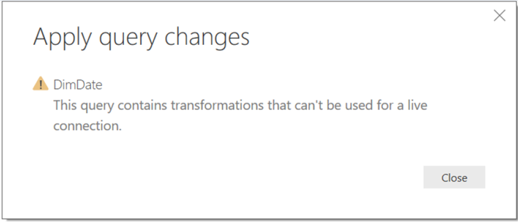
    • When Direct Query is used you can no longer do many of the data mashup actions in the “Edit Queries” section of Power BI. It is assumed that you will have already done this in the backend. You can do simple actions such as removing columns, but don’t expect to be able to manipulate the data much. The Query Editor will allow you to make transformations, but when you try to load to the model you will most likely get an error that looks something like this
    Direct Query Error
    Direct Query Error 
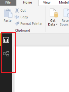
    • The data tab is also disabled in the model layer and thus you need to make sure that all the formatting and data transformations are completed in the source.
    Data Tab no longer present
    Data Tab No Longer Present
    • You can do some minor adjustments to format, but this could be a heavy restriction if you don’t have access to the data source.
    • There are performance impacts to the report that need to be taken into consideration. How large is the audience that will be interacting with the report? How busy is the source system, are there other processes that could be impacted?
    • Troubleshooting skills in source system language
    • Multiple applications required to adjust data ingestion and formatting

    Pros:

    • The Direct Query connection does not store any data. It constantly sends queries to the source to display the visuals with the appropriate filter contexts selected.
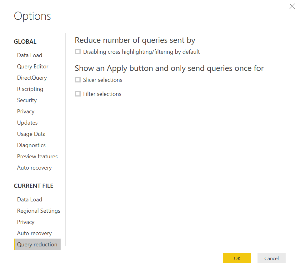
    • In the November 2017 release there is a new capability in Power BI allows you to reduce the traffic and enhance this connection method exponentially. The feature is called Query reduction, and allows you to enable an “apply” button on a slicer or filter. The benefit with this option is that you can set all your selections of a filter prior to Power BI executing the query. Before this feature was available, every selection you made would fire off a query to the source database. To enable this feature, go to File -> Options and Settings -> Options -> Query Reduction you will find these options to help with Direct Query Performance.
    Query Reduction Options
    Query Reduction Options

    Note: This enhancement greatly increases the performance of a Power BI report against the data source, but be aware that there could be poor query performance, or aspects of the solution that would require troubleshooting in the data source depending on what queries are being passed. This would require understanding of how to performance tune the source.

    • Deployment of the Direct Query connection requires the use of the gateway previously called the Enterprise Gateway. Note that the Enterprise Gateway is different than the personal Gateway.
    • No data is ingested into the model using Direct Query thus, there is no need to schedule a refresh. Once the dataset is connected to the Gateway, the data source feeds information to the report as the user interacts with the report.
    • It will always show the latest information when you are interacting with the report.

    Direct Query is a powerful connection type in that it produces the most up to date data. However, as we have seen, it does come with some considerations that need to be taken into account. The Pros and Cons of the connection mostly revolve around whether or not the end user can understand and deal with potential performance issues, updating data retrieval processes, and understand the downstream implications of a wider audience. Typically, Direct Query is used in extremely large datasets, or in reports that require the most up to date information. It will most likely always perform slower than an import connection and requires an understanding of tuning and troubleshooting of the data source to alleviate any performance issues.

  • Start of Month DAX Calendar

    Start of Month DAX Calendar

    While on a recent project I needed to build a variation of the DAX date table.  In my previous post, found here Creating DAX Date Tables I was built a date table for every day of the month for multiple years.  I’ve only ever needed to consume a fully populated date calendar, but in this instance because the data I was collecting was already aggregated to the first of the month I only needed a date calendar with each month’s start date.  After some playing around with my previous DAX functions I think I was able to come up with an elegant solution.

    Let’s get into it.

    Let’s begin by making a basic table.  Open Power BI Desktop, on the Modeling ribbon click New Table.

    Enter the following code:

    Dates = 
      GENERATE ( 
        CALENDAR ( DATE ( 2017, 1, 1 ), DATE ( 2017, 12, 31 ) ), 
        VAR currentDay = [Date]
        VAR day = DAY( currentDay )
        VAR month = MONTH ( currentDay ) 
        VAR year = YEAR ( currentDay )
      RETURN ROW ( 
        "day", day, 
        "month", month, 
        "year", year )
      )

    This will produce our standard table from January 1st to December 31st, 2017 with every day populated in between.  In, addition we get numerical values for Day, Month and Year.

    Note: This table is producing a list of dates using the Calendar DAX function then iterating row by row to calculate each numerical value for the Day, Month and Year.

    Add the Table visual with the following Values from our created DAX table.

    Dates Table
    Dates Table

    Note: When you drag over the field labeled Date the field will be naturally added as a Date Hierarchy.  To remove the Date Hierarchy, you have to click the little drop down arrow next to the word DATE and select the word Date in the drop down menu.  This will remove the Year, Quarter, Month and Day date context from the visual.

    The date calendar we made has every date, but we want only the first of each month.

    Lets build a new table by following the previous steps and adding the following:

    Start of Month Dates =
      GENERATE (
        GENERATESERIES(1,12),
        VAR inc = [Value]
      RETURN ROW (
        "date", DATE(2017,inc,1)
        )
      )

    Add the Table visual to the report page and add the following fields:

    Start of Month Date Table
    Start of Month Date Table

    Note: I already removed the Date Hierarchy using the instructions listed above in the previous note.

    This new DAX Date table is first generating a list of numbers 1 to 12 one for each month.  Then it iterates through the list and produces a date using the Date function were we manually provide the Year, and the day.  You can see the Generate function produces a column of data called [Value].  The variable denoted by VAR inc is capturing the number for each month.  So, now what if we want to produce more than one year of dates?  Super simple, just change the generate series from 1 to 12 to 1 to 48.  This will produce three years of dates.

    Change your Start of Months Dates to the following:

    Start of Month Dates =
      GENERATE (
        GENERATESERIES(1,48),
        VAR inc = [Value]
      RETURN ROW (
        "date", DATE(2017,inc,1)
        )
      )

    With one number change we can produce 4 years of dates.

    Four Years of Dates
    Four Years of Dates

    Cool, let’s go a little further.  Just in case we need it we can also produce a list of dates that contain the end of the month.  Add the following your Start of Month Dates with the following DAX table (don’t forget the comma on line 1 in the ROW function):

    Start of Month Dates =
      GENERATE (
        GENERATESERIES(1,48),
        VAR inc = [Value]
      RETURN ROW (
        "Date", DATE(2017,inc,1) ,
        "Month End", EOMONTH( DATE(2017,inc,1), 0)
        )
      )

    We have added a new column to note the end of each month.

    Date Table with Start and End Columns
    Date Table with Start and End Columns

    Well, thanks for following along.  In my use case this start of month date table was exactly what I needed.  I thought this was a handy little DAX table, and I hope you have found this helpful as well.  Be sure to share this post if you found this helpful.