Tag: CSV File

  • Load Multiple Excel (xls or xlsx) Files

    Load Multiple Excel (xls or xlsx) Files

    Previously we’ve done a tutorial on loading multiple text files within one query.  This is nice, however we will also need to import multiple Excel files.  First, to understand the procedure of querying multiple excel files you have to understand the basics between the CSV (comma separated values) file and an excel (.xls or .xlsx) files.  In a CSV file you have only one data set.  The beginning of the file starts with values and separates each file with a “,”  a carriage return starts a new row of data.  This is an easy and efficient way to store millions of rows of data.  By contrast the excel file is way more complicated.  Excel files can have multiple sheets of tables of data.  Think of this as a stack of CSV type files.  For example if you have an excel workbook with three sheets of data, Sheet 1, Sheet 2, Sheet 3.  You can think of those three sheets as grid of data, similar to the CSV file.  The multiple sheet aspects of an excel file makes the data ingestion into PowerBI a little bit more complicated.  To add to the complication, when you loading data from either multiple sheets, or selecting a specific out of many sheets of data.  For illustration purposes imagine working with two excel files with three sheets each, 2 x 3 = 6, a total of 6 sheets of data, or what I will call “pages” of data.  This is why it is more complex to load excel files than CSV files.

    Note: If you want to learn how to load multiple CSV files visit this tutorial.

    Not only do you have to figure out what data you want to ingest on the page you must all tell PowerBI which sheets do you want to look at, and from which excel file.  If that was to many words think of loading the following data sample:

    Workbook 1 – Year 2000 Olympic Medals

    • Sheet 1
      • Olympic Medals Table
        • Rank
        • Country
        • Gold
        • Silver
        • Bronze
        • Total
    • Sheet 2
    • Sheet 3

    WorkBook 2 – Year 2004 Olympic Medals

    • Sheet 1
      • Olympic Medals Table
        • Rank
        • Country
        • Gold
        • Silver
        • Bronze
        • Total
    • Sheet 2
    • Sheet 3

    The data structure for both workbook 1 and 2 are similar but the names of the files are different and there can be multiple pages.

    To resolve this we will have to write a M language function that will load each file as a function.  This will be done in later in the tutorial.

    Here is the data source information for Olympic medals won by each country from 2000 to 2012, download here.  Inside the Medal Count zip file are four xlsx files, extract them to your desktop.  Move the files into a folder on your desktop labeled Medals.
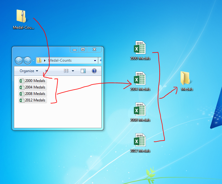
     

    Medals Folder
    Medals Folder

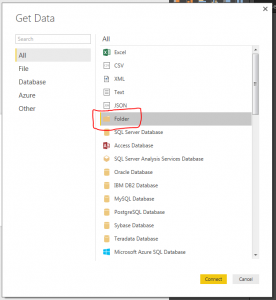
    Now, open up PowerBI,  We will begin shaping our data to load all the excel files.  On the Home ribbon click on the Get Data button.  Select Folder on the right side and click Connect.
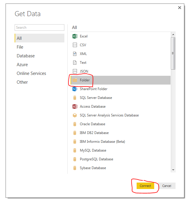
    Get Folder Data
    Get Folder Data

    Next select the folder path that you want acquire the files from, Click OK to continue.
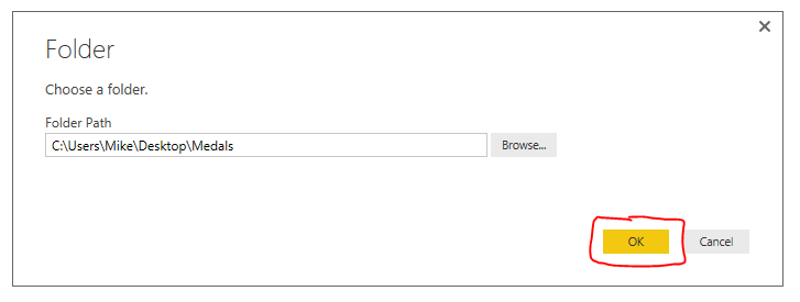
    Load Folder Screen
    Load Folder Screen

    Next we are presented with the loaded files within our selected folder.  Click Edit at the bottom of the screen to proceed.  The Query Editor window will now open.  Select the first two columns labeled Content, and Name.  With those two columns selected right click on the header and select Remove Other Columns. This will remove all the useless data associated with the files.
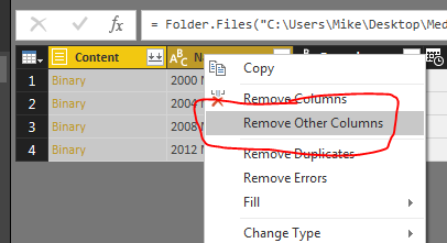
    Remove Other Columns
    Remove Other Columns

    Click the Add Column ribbon and press the Add Custom Column on the left side of the ribbon.
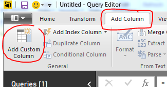
    Add Custom Column
    Add Custom Column

    Name the new column ExcelFileLoad and enter the following equation.
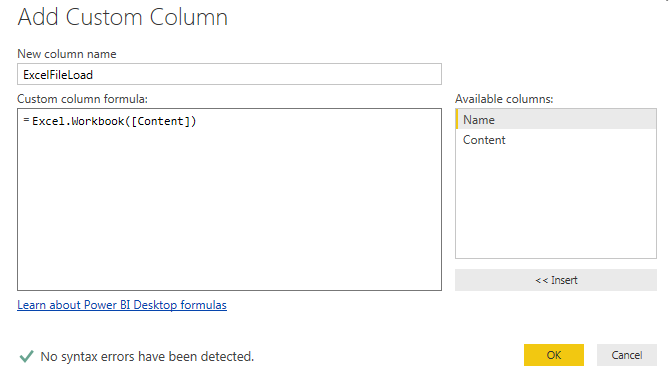
    Excel.Workbook Equation
    Excel.Workbook Equation

    Note: Once you type “Excel.Workbook(” you can click on the column labeled Content on the right side of the screen to have the name automatically added.  This is useful when you have many many columns to choose from or if there naming of those columns becomes complex.  This way you won’t type in the column name incorrectly.

    Click OK to proceed.  Notice we now have a new column called ExcelFileLoad.  Next click the Expand button (the one with the arrows) located at the right of our newly added column. Click OK to proceed.
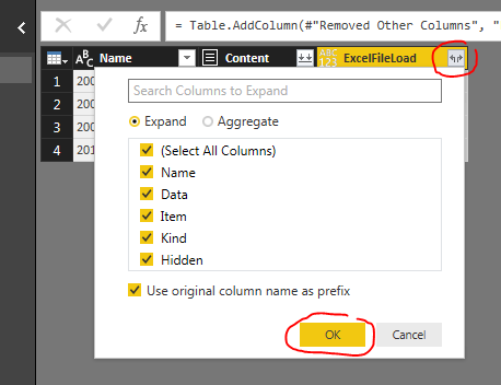
    Expand Column Button
    Expand Column Button

    Now we have a new column labeled ExcelFileLoad.Data, which is the data contained in our excel files.  Now click in the Grey Area next to the word labeled Table.  This will open up the file and reveal the information present in the file.  Notice that we can see the headers and the data in our file.  Row 1 contains the headers of each column.  Rows after row 1 contains the medal data.
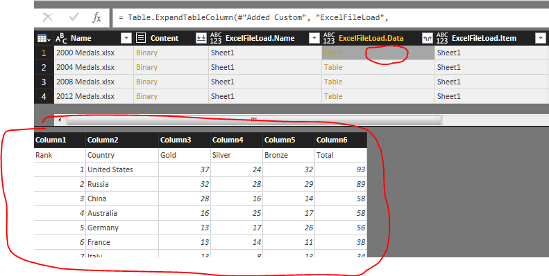
    View Data of File
    View Data of File

    Next select the columns labeled Name and ExcelFileLoad.Data and right click on the column header, then select Remove Other Columns

    Remove Other Columns Again
    Remove Other Columns Again

    On the Add Column ribbon click Add Custom Column again.  Name the column PromoteHeaders and enter the following formula. Click OK to proceed.
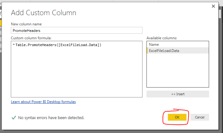
    Promote Headers Step
    Promote Headers Step

    Clicking again on the grey area in our newly created column reveals our tables with promoted headers.
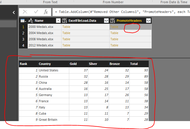
    View of Data with Promoted Headers
    View of Data with Promoted Headers

    Next click the Expand Button, un-check the Use original column name as prefix and click the OK button to proceed.
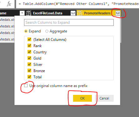
    Expand Data
    Expand Data

    Remove the following columns, ExcelFileLoad.Data, Rank,  and Total, bu right selecting the columns and right clicking on the header and selecting Remove Columns.  Now we want to parse out the year name from the Name column.  To do this click on Name Column.  Then click the Transform ribbon and click the Extract button, then select First Characters from the drop down menu.

    Extract First Characters
    Extract First Characters

    In the Extract First Characters menu enter the number 4 and click OK to proceed.
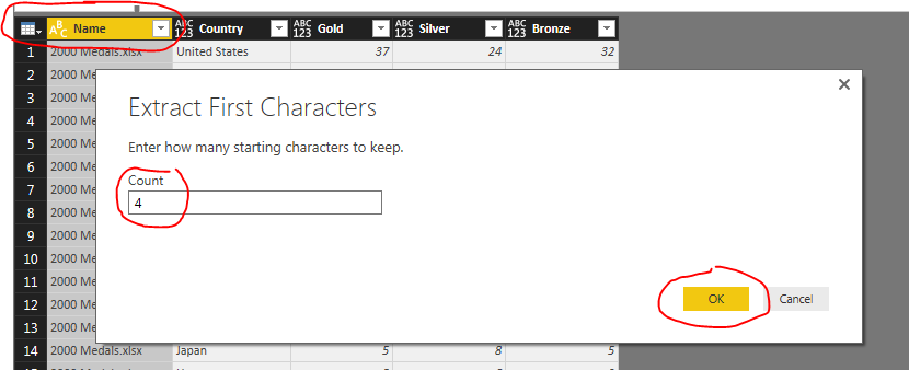
    Extract First 4 Characters
    Extract First 4 Characters

    Change the following columns to whole numbers: Name, Gold, Silver, Bronze.  Do this on the Transform ribbon in the Data Type drop down.
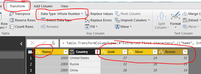
    Change Data Types
    Change Data Types

    We are now ready to load all the data.  Rename the Query to Medals, click the Home ribbon and select Close & Apply.
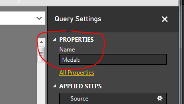
    Name Query
    Name Query

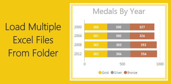
    And there you have it.  We have successfully loaded four excel files into one query.

    Bonus: for added flare add the following measure.

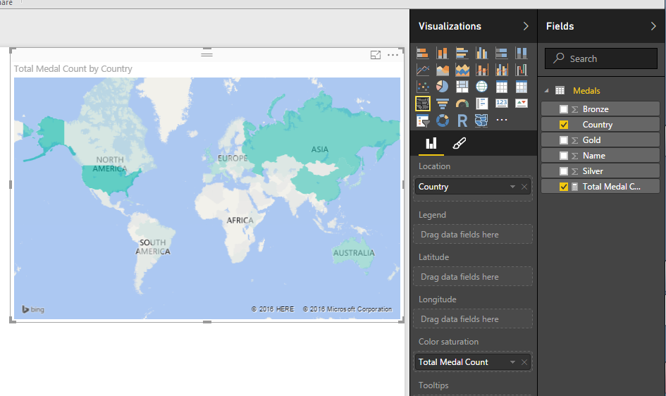
    Total Medal Count = sum(Medals[Gold]) + sum(Medals[Silver]) + sum(Medals[Bronze])

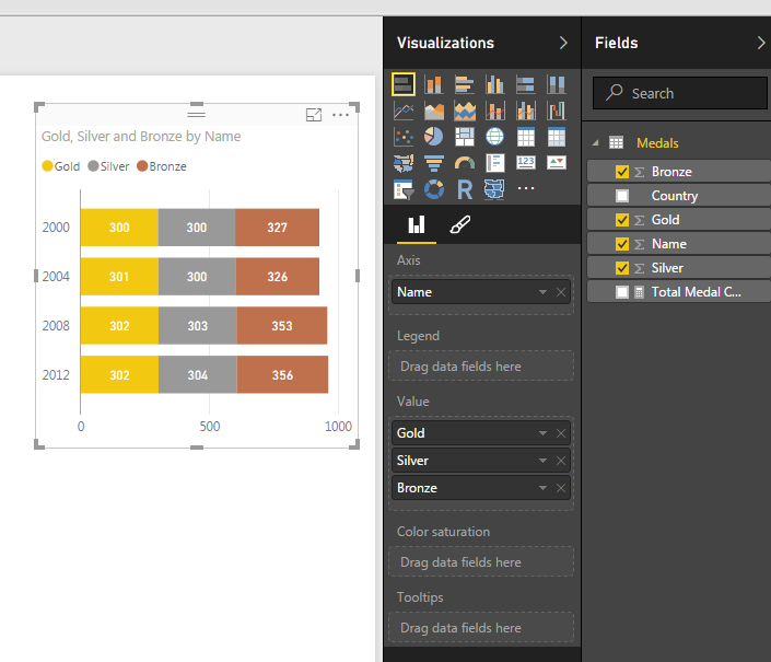
    Now you can add the following Visualizations.
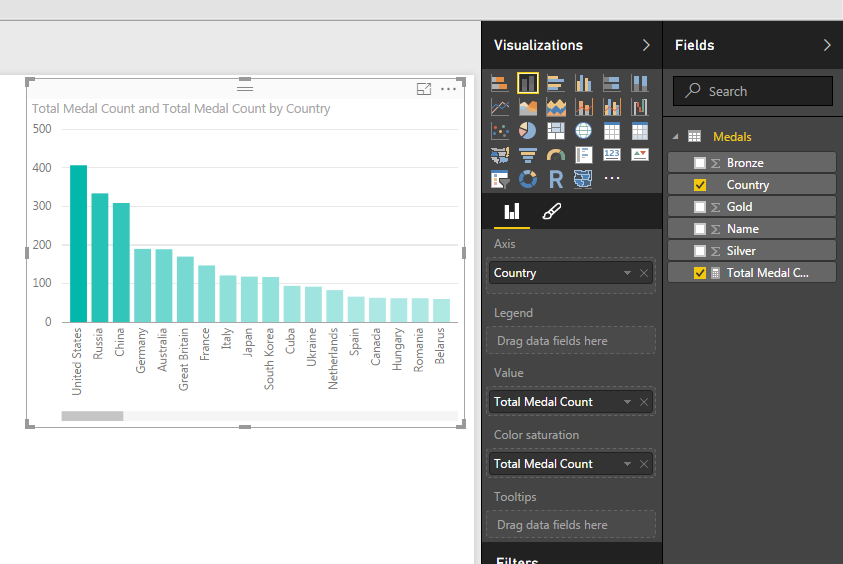
    Bar Chart Visual
    Bar Chart Visual
    Stacked Bar Chart
    Stacked Bar Chart
    Map Visual
    Map Visual
  • Loading Data From Folder

    Loading Data From Folder

    Let me setup a scenario for you.  You get a data file from an automated system, it has the same number of columns but the data changes for every new file.  Being the data savvy person that you are you’ve spent some time working in excel to make a template where you can copy your new data into and then automatically all your equations and graphs magically work.  You pat your self on the back and happily send out your fantastic report to everyone you know.  Then tomorrow when the data comes to you again you repeat the same process over again.  Still enamored by your awesome report, you send it out again knowing you have saved your self so much time not having to do the analysis or creation of your reports over and over again.  Now, fast forward 3 months.  That stupid report shows up again, and now you have to lug all that data from file to file and begrudgingly you sent out your report.  Thus, is the store of the analyst.  You love data, but you hate it as well.  Well in this tutorial I’ll show you how to remove some of the pain of that continual data loading process by loading new data from a folder.

    My previous post (found here) talks about loading data from a folder.  In this tutorial we will add some logic to this method that will look at a folder but only load the most recently added item from that folder.

    Data for this tutorial is located this link Monthly Data Zip File.  This data in the ZIP file is a monthly data sample from Feb 2016 to April of 2016.

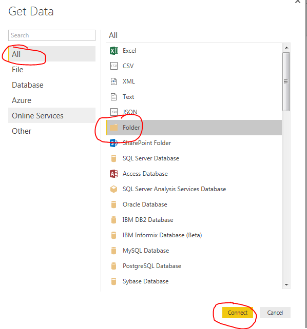
    Download the zip file mentioned above and extract the Monthly Data folder down to your desktop.  Open up PowerBI Desktop and click on the Get Data button and select All on the left side.  Click on the item labeled Folder and click Connect to continue.

    Get Data from Folder
    Get Data from Folder


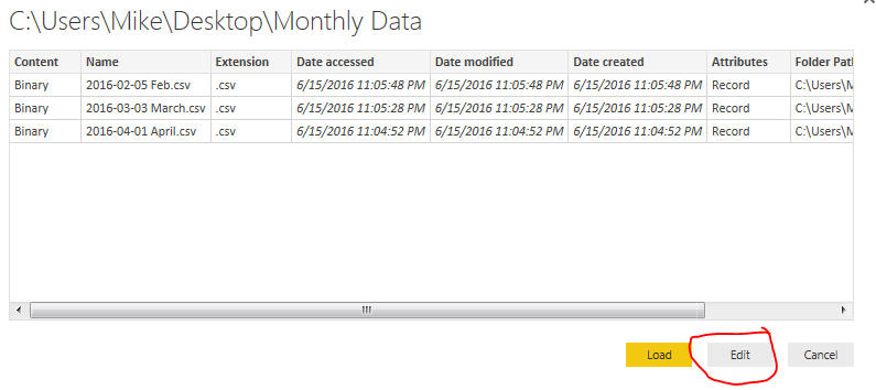
    Select the newly unzipped Monthly Data folder that should be on your desktop.  Click OK to continue. Upon opening that folder location you will be presented with the multiple files.  Click Edit to edit the query.

    Edit Query for Folder Load
    Edit Query for Folder Load

    Now you are in the Query Editor.  This is where the fancy query editing will work to our advantage.  We could load all the data into one large query.  However, depending on the size of your data sets or how you want to report your data this may not always be desirable.  Instead you may only want data from April, then May when the new data is sent next month.

    Thus, our first step to start pairing down the data will be to first filter the files in sequential order.  In this case because I have named the files with a Year-Month-Day format I can sort the files according to their names.

    Note:  When using PowerBI desktop it is a good practice to name the files  beginning with a YYYY-MM-DD file name.  This makes it really easy when sorting and ingesting information into PowerBI.  I have used other columns of information such as Date Accessed or Date Created before but have gotten inconsistent results as these dates can change depending on when a file was moved or copied from one place to another.

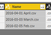
    Click the drop down next to Name and sort the files in Sort Descending.

    Name in Descending Sort
    Name in Sort Descending

    This places the files with the most recent file at the top of the list.

    File List in Descending Order
    File List in Descending Order

    Next click on the Keep Rows button on the Home ribbon, select Keep Top Rows.

    Keep Top Rows
    Keep Top Rows

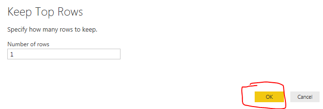
    Enter the number when the popup appears.  Click OK to continue.

    Keep Top Rows Menu
    Keep Top Rows Menu

    Now you’ll notice you have only one file selected which is our latest file from April.  Click the Load File button found in the Content column.

    Load File Button
    Load File Button

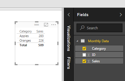
    We have completed the activities in the Query Editor and can now load the data.  Click Close & Apply found on the Home ribbon.  All our April data has loaded.  by making a simple table we can now see all the data that was just loaded.

    Loaded Data from April
    Loaded Data from April

    Now we will remove some data from our desktop folder labeled monthly data.  Open the folder on the desktop labeled Monthly Data and delete the filed labeled 2016-04-01 April.  You should now have a folder labeled Monthly Data with only two files in it, one for Feb and one for March.

    Two Files Left
    Two Files Left

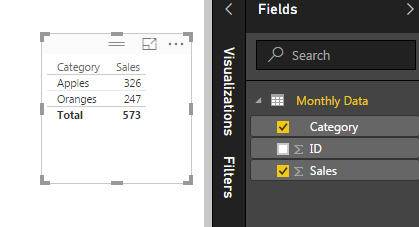
    Return back to Power BI Desktop and click the Refresh button on the Home ribbon.  Notice now how all our data has changed.  We are now looking at the March data because it is the most recent file in our folder based on the file name.

    March Data Load
    March Data Load

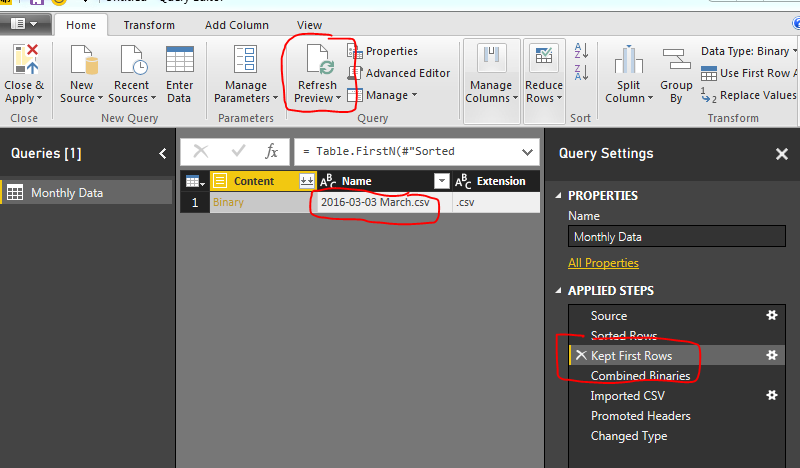
    To verify this we open the query editor (Click the Edit Queries on the Home ribbon).  Click Refresh Preview on the Home ribbon and finally select the Applied Step called Kept First Rows.  This will reveal the month of March as our data source.

    Month of March Loaded
    Month of March Loaded

    Now, every time you add a new file to our folder and refresh PowerBI the latest file (based on the naming convention we talked about earlier) will always be loaded.

    Note: This method works great when your data source is coming from an automated system.  The file format must always be the same for this to work reliability.  If the file naming convention changes, or the number of columns or location of those columns changes then the query will most likely fail.

    Good luck and thanks for following along.

  • Folder of Files Loaded to Power BI Desktop

    Folder of Files Loaded to Power BI Desktop

    Ok, I’ve got to be honest the first two tutorials (Loading Excel Files, Loading CSV Files) were only there to get things kicked off. Now we are getting to some of the good stuff.

    When I first saw this feature in Power Query for excel I nearly had a conniption.  My first thought is this is going to CHANGE EVERYTHING, and to be perfectly honest it has. My entire view of Excel and Power BI has been shaped by this simple but powerful idea; Automated Data Loading.

    In all my years as an engineer I would have to constantly copy and paste data from one excel file to another. Then perform some transformations just to produce a bar chart or a line graph, uggh.  This is slow and boring.  I was really good at being boring, and I felt like I was able to become quite ingenious by writing macros and automating parts of my data transformations.  Now I have seen the light,  The simple ability of being able to load a group files from a folder is AWESOME!  Had I had this feature in my engineering days I could have saved so much time.  So in true homage of my engineering roots this post is for you, the all mighty data hungry engineer.

    Alright, enough of be babbling, Lets get to it.

    Materials for this Tutorial:

    • Zip file with (3) three excel files download Data Set.
    • Power BI Desktop (I’m using the March 2016 version, 2.33.4337.281) download the latest version from Microsoft Here.

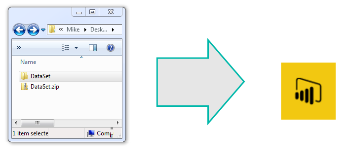
    Lets start off by downloading the Data Set and unzipping the file to a folder called DataSet.  For this demo I unzipped the files to my desktop folder.

    UnZipped Files
    Location for UnZipped Excel Files

    Next we will open up Power BI Desktop.  On the Home ribbon select the Get Data button.  The Get Data window will be presented and this time we will select the Folder icon in the menu.

    Get Data Folder
    Get Data Folder Icon Selection

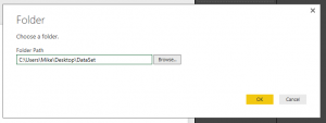
    Click the Connect button at the bottom right of the screen.  A folder window will display.  This is where we will select the location of our data in the folder we unzipped earlier.  Click OK once you’ve selected the location of the folder.

    Folder Path
    Folder Path Location

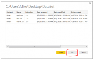
    The next window to open shows the files that Power BI Desktop is able to see in the folder location.  Normally we would press Load and move forward but in this case we want to further manipulate our query to load the data.  Therefore, Click the Edit button to modify the query to load data.

    Folder Location
    View of Files in Selected Folder

    We are now in the Query Editor.  This is where we can manipulate the incoming data before we visualize it.

    Note:  The Query Editor is a graphical representation of the M-language which is used to load data.  Each button press in the Query Editor performs a transformation to your data.  Each step writes a little line of code that handles the transformations.  To see the code Click the View ribbon then click the button labeled Advance Editor.  For more documentation on the M language look at the Microsoft documentation located here.

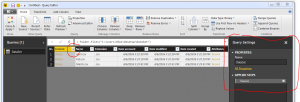
    Here is an image of the files we loaded in from our folder location in the Query Editor.

    Query Editor
    View of Query Editor

    The next step is to combine all the files into one combined data model.  To do this click the Double Down Arrows that are circled in red on the left side in the column called content.  

    Note: I also circled the Query Settings in Red on the right.  The Query Settings window will become very useful, especially when trouble shooting a query.  You will notice as we make additional data transformations more steps will accumulate in the query settings.

    We now have a final view of all the data from each of the three CSV files.

    Data Model
    Loaded Files into the Data model

    The file needs a little clean up to remove some unwanted data rows.  Notice now that we have loaded all three files.  In each file we had a header row.  Now in our data model we have three rows with headers.  We want to use the first row as column names.  To do this, Click the Use First Row as Headers button on the Home ribbon.

    Header Row
    Use First Row as Headers

    Also, notice there are rows of data that contain the initial header rows from the other two files.

    Other Headers
    Header Rows from Other Two Files

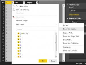
    Now we will apply a filter to remove these rows.  Click the Arrow in the ID row.  This will present a menu.  There are various transformations on this screen, you can sort a row in Ascending, or Descending order, Filter out text items, etc…

    Filter ID Row
    Filter for ID Row

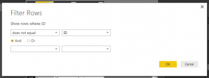
    Click Text Filters and select Does Not Equal and enter ID into the filter.  Click OK to proceed. This will add a step to remove any row that had ID listed in the ID column.

    Filter Rows
    Filter out the Text “ID” from column

    We have transformed our data and now have cleaned the data and it’s ready for use.  Click Close and Apply to load the data to the data model.  Now the data is ready for visualizations.  Thanks for following along.

    Make sure you take some time to share if you enjoyed this tutorial.

  • Import CSV file to Power BI

    Import CSV file to Power BI

    This post is going to be similar to my previous post about Getting Data.  I figure we better cover some of the basics before going crazy with deeper topics.

    Materials for this tutorial:

    • CSV file with some random data, linked here: SampleData in CSV format
    • Power BI Desktop (I’m using the March 2016 version, 2.33.4337.281)

    After I read the previous version I thought it would be helpful to put the materials up at the top and what version I was using.  If you didn’t know Microsoft has been very active in the development of PowerBI.com and Power BI Desktop.  Right now there are weekly updates to PowerBI.com and monthly updates to Power BI Desktop.

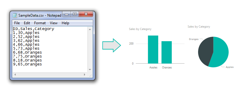
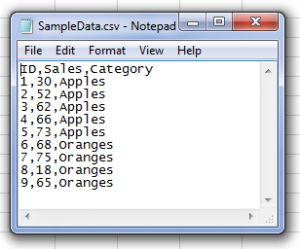
    Starting off like before here is a sample of the data from the csv file.  I’m showing the data in notepad to prove it is a comma separated value file (hence the CSV name).

    csvfile
    CSV File opened in Note Pad

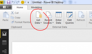
    Alright, lets go get some data.  Open up Power BI Desktop.  Click on the Home ribbon.  Select the Get Data icon.

    Get Data Button
    Button for Get Data

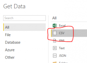
    Now the Get Data window will open.  Next, select the second item labeled CSV from the top of the list on the right.

    Get CSV selection
    CSV selection in the Get Data screen

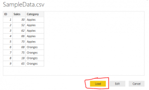
    Click the Connect button at the bottom right hand of the Get Data screen to proceed to the next screen.  Now the open window will let you navigate to the CSV file you would like to import.  Click the Open button at the right of Open window to load the CSV file.  Finally you’ll be presented with the data view of the contents contained inside your CSV file.

    View Of CSV Data
    View of CSV Data file

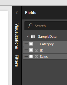
    Once loaded we now have our view of all the columns of data in the Fields viewing pane on the right.  From here we can build our visuals.

    Loaded CSV Columns
    Loaded Columns from CSV file load

    Now, lets throw together a quick visual of the data.

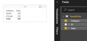
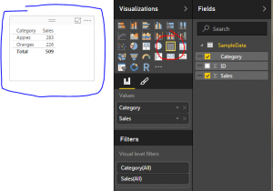
    Start by clicking the check box next to the label titled Category and then click the box next to the label titled Sales.  This will automatically populate a table with the categories in the first column and the sales for each category in the second column.

    Table Visual
    Table of Data

    To open up the Visualizations bar click on the word Visualizations.  This will present all the information relating to the visuals. Upon opening up the visualizations pane there is a small yellow square showing you which visual is selected.
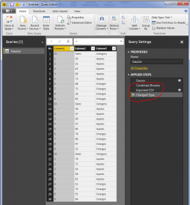
    Selected Visual
    Showing the Selected Visual

    Note: The blue pen highlighting shows the selected visual on the page.  As you build more complex visuals there will be multiple visualizations on your page.  When you select a specific visual, all the properties in the Visualizations Bar show all the properties for the selected visual.  The Table visual is highlighted by the red highlight circle.

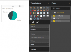
    To change our selected visual to a new visual we will simply select a new icon in the Visualizations bar. Click the icon that looks like a pie chart.

    Pie Chart
    Pie Chart Visualization

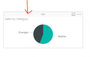
    Cool, but what if I want more awesomeness on my page.  No problem.  Let’s copy our visual.  You can do this by selecting the visual.  To know it is selected look for the slight grey bar at the top of the visual.

    Gray Bar on Visual
    Gray Bar denoting that visual is selected

    Copy the visual by using Ctrl + C.  Click any where on the white space on the page.  This will deselect the current visual.  Then paste an identical version of the visual by using Ctrl + V.

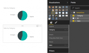
    Two Visuals
    Copy and Paste of new Visual

    Ta-da! Now we are really getting somewhere.  Two Amazing visuals, well not quite.  Two identical visuals isn’t very compelling.  Lets change one of the visuals to a different visual.

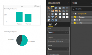
    Select the top visual by clicking on it.  Then select the Stacked Column Chart which is the second icon from the left in the top row.  Selecting this icon will change the visual.

    Bar Chart
    Bar Chart Visual

    And there you have it.  You’ve imported a CSV file and generated two visuals.  Nice job.

    Hope you enjoyed this tutorial.  Leave comments if you have questions or if you want to see something else in a tutorial. If you like what you see please share this post on your selected social network of choice below.