April 7, 2016
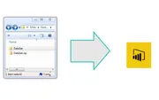
Folder of Files Loaded to Power BI Desktop
Learn how to load multiple files from a folder into Power BI Desktop using the powerful automated data loading feature that will change how you work with data.
Tag
3 posts
April 7, 2016
Learn how to load multiple files from a folder into Power BI Desktop using the powerful automated data loading feature that will change how you work with data.
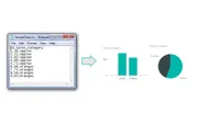
April 1, 2016
Learn how to import CSV files into Power BI Desktop, create tables and charts, and copy visuals to build compelling data visualizations.
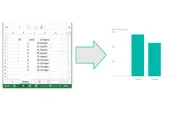
March 29, 2016
Learn how to load data from Excel into Power BI Desktop with this simple step-by-step tutorial covering the Get Data function and basic visualizations.