
One of the most important concepts to learn within Power BI Desktop is how to build a Data Model.
Note: In simple terms the Data Model is data that is collected from the get data function. In your data model you can build multiple queries. This data is stored in the file. The data storage is very efficient as the data compressed down to approximately a 4:1 ratio. 1000 KB file will compact down to approximately 250 KB when loaded into Power BI. From my current understanding all data is loaded into the memory of the computer. Thus, if you are having performance issues it could be in part due to the RAM of your computer.
As you begin to craft more data models you will learn little tips and tricks along the way to make an efficient Data Model for your visualizations. I have found that the most challenging part of building the data model is structuring the data in a way that will make your selected visual make sense. This may mean you need to add a measure or a calculated column or a ranking to a data set. Alright lets get started.
Here are the Resources for this tutorial:
- Power BI Desktop (I’m using the March 2016 version, 2.33.4337.281) download the latest version from Microsoft Here.
- We are going to work through the Power BI Desktop file that we built in the Loading Excel Files Into Power BI Tutorial. You can follow the link to create the Power BI Desktop (pbix) file in the tutorial. For convenience, the completed file can be downloaded here: Import Excel Tutorial.
I’m going to start off by extracting the Import Excel Tutorial.zip file to my desktop. Once the file has been extracted we can open the containing folder. In this folder there are two files the source data in the excel file and the Power BI Desktop file.
Note: A Power BI Desktop file has a .pbix file format ending.
Open the Import Excel.pbix file. First click the Home ribbon and then click the Refresh button. Most likely there will be an error similar to the following message.

This type of message occurs when you refresh a query and the file is missing or can’t be found. This is because when i originally built the Power BI Desktop tutorial the excel file that is supply the information was located on my desktop. This is a common problem when you build connections to local files stored on your computer. If you move a file into a different folder then the connection will break.
To resolve this close the message window by clicking Close. on the Home ribbon click the Edit Queries button. The Query Editor window will be presented. In a large yellow bar in the data view portion of the window (circled in red) is the error message.
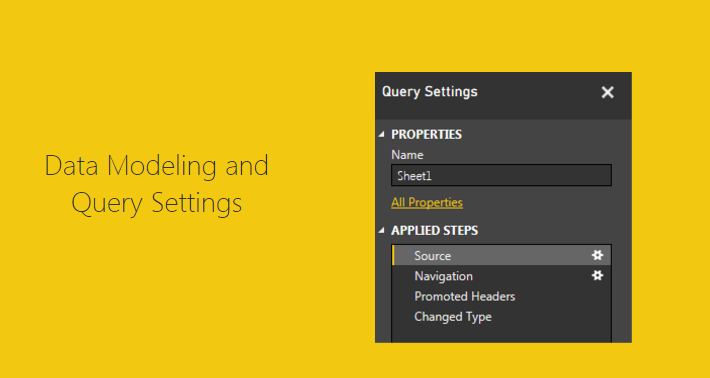
Note: Circled in blue is the Query Settings window. This window is the window for all the applied steps to transform the data. You can change the name of the query in the name box. From the view we have selected we can see that the step entitled Changed Type is currently selected (seen circled in blue).
Click the grey button labeled Go To Error which is found in the yellow error box.

Upon clicking the Go To Error button the selection in the Query Settings button to the Source Step. This is where the query has failed. More information about the failure is shown in another yellow error box. This time click Edit Settings in the error box.

Now we have the Load Excel file window prompt open. In this window Click Browse, navigate to where you extracted all the files downloaded earlier in the tutorial and select the excel document entitled Book1. Click Open and the new file location will be loaded into the Load Excl Window. Click OK to complete the settings change.

Now the data is correctly loaded into the data model. Notice we are still on the step called Source. Take some time to click through each step, Source – Navigation – Promoted Headers – Changed Type. As you click on each step you can see how the data is transforming.
To see the code that is being used to make each step click the View ribbon and check the little box entitled Formula Bar. This will make a formula bar appear. When you click on a step the formula bar will reveal the code needed to complete the selected step.

We can now see the equation, which is similar to how you would write an equation in excel. The code in the Changed Type step is here:
= Table.TransformColumnTypes(#"Promoted Headers",{{"ID", Int64.Type}, {"Sales", Int64.Type}, {"Category", type text}})
The equation is using the M language to transform the data. More information on the usage of the M language can be found here.
Note: Couple of pointers about the data shown in the formula. The function is called Table.TranformColumnTypes. The source of the data is a variable called #”Promoted Headers”. The pound sign and the words following in quotations is how the M language passes variables that have a space contained in the language. Since the prior step has the name “Promoted (space) Headers” the program has to add the pound sign and the quotation marks. If there is no space in the naming convention such as “PromotedHeaders” then only the PromotedHeaders would be seen in the code and the pound sign and quotes will be gone. See modify coded when I remove the space from the Promoted Headers applied step.
= Table.TransformColumnTypes(PromotedHeaders,{{"ID", Int64.Type}, {"Sales", Int64.Type}, {"Category", type text}})
Notice the the pound sign and quotations are missing.
The second part of the formula is an array which has been written out in curly brackets:
{
{"ID", Int64.Type},
{"Sales", Int64.Type},
{"Category", type text}
}
I changed the code by adding line returns to make it easier to read. The coded array has beginning bracket and an ending bracket. Each parameter is contained in it’s own curly brackets and separated with a comma. The array is a 2 x 3 array, it has 3 rows and two data points on each row, just like a matrix. The first data point is the column name. In the first row the column that is being address is called ID. The data transformation parameter is called Int64.Type. This means that the data is an integer type 64 bit. This repeats for each row until all parameters have been addressed.
So there you go, we have opened up a query repaired it and learned a little about the formula bar.
As a side note, as you build queries each button press that you make on the various ribbons in the Query Editor will make a minimum of one step the in the Query Editor.
Hope you enjoyed this short tutorial about the Query Editor. Make sure you share below if you liked it.