Use Multiple Connections Between Tables
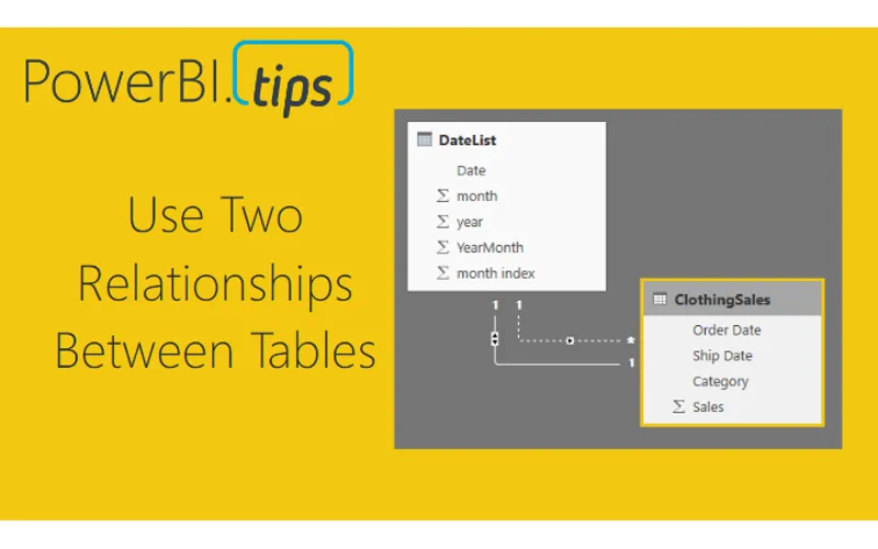
For those of you who work in supply chain management this tutorial will be right up your alley. In my previous job position I had a lot of interaction with our shipping department. We would look at when orders were placed from the customer, and conduct a comparison to what orders were actually shipped or cancelled prior to shipment. Our analytics team would produce reports and metrics to our customers about orders and shipment information.
In an ideal world, every product ordered on the purchase order would be shipped and some point in the future. But, as we know, in the real world this isn’t always the case. Orders get cancelled, products get re-ordered, challenges happen, and therefore we would need to track all these changes. In our shipping analytics group, the team would pull data from our shipping system with columns similar to the following:
Order Date, Ship date, Product type, and Shipped QTY
Sometimes you want to sum the data by the order date, and in other cases you want a total by the shipped date.
In this example, we will walk through making a measure that uses the DAX formula USERELATIONSHIP. To learn more about this function from the Microsoft documentation follow this link.
Open PowerBI Desktop, click the Get Data button on the Home ribbon and select Blank Query. Click Connect to open the Query Editor. On the View ribbon click the Advanced Editor button. While in the Advanced Editor paste the following code into the editor window, click Done to complete the data load.
Note: If you need some more help loading the data follow this tutorial about loading data using the Advanced Query Editor. This tutorial teaches you how to copy and paste M code into the Advanced Editor.
let
    Source = Excel.Workbook(Web.Contents("https://powerbitips03.blob.core.windows.net/blobpowerbitips03/wp-content/uploads/2017/06/Clothing-Sales-Ship-Order-Dates.xlsx"), null, true),
    ClothingSales_Table = Source{[Item="ClothingSales",Kind="Table"]}[Data],
    #"Changed Type" = Table.TransformColumnTypes(ClothingSales_Table,{{"Order Date", type date}, {"Ship Date", type date}, {"Category", type text}, {"Sales", Int64.Type}})
in
    #"Changed Type"
Your loaded data should look like the following:
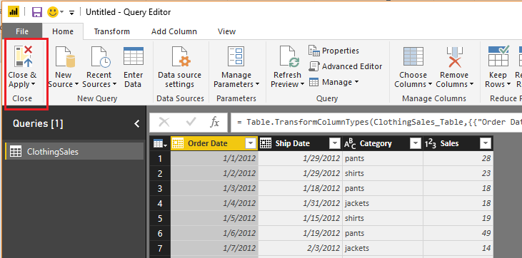
Sales Data Load
Click Close & Apply on the Home ribbon to load the data into the data model.
We will want to create two measures, one that performs a calculation on the Order Date column, and one on the Ship Date. To do this we need a date table to populate all the dates needed for this data set.
We can do this by creating a DAX date table.
On the Modeling ribbon click New Table.
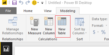
New DAX Table
In the formula bar enter the following.
DateList = GENERATE ( CALENDAR ( DATE ( 2012, 1, 1 ), DATE ( 2017, 12, 31 ) ), VAR currentDay = [Date] VAR startYear = 2012 // we know this by looking at our data VAR month = MONTH ( currentDay ) VAR year = YEAR ( currentDay ) RETURN ROW ( “month”, month, “year”, year, “month index”, INT ( ( year – startYear ) * 12 + month ), “YearMonth”, year * 100 + month ) )
Note: This DAX formula is building a date table, for each row we are building the columns, Month, Year, Month Index, and an integer for YearMonth index. This is a simple way to repeatedly create a date calendar based on your data.
Great, we have completed the data loading. Now, we need to link the date table to the Clothing Sales data. To do this click on the Relationships button on the black navigation bar located on the left side of the screen. Then Click & Drag the Date column from the DateList table to the Order Date column of the ClothingSales table. This will create a one to one relationship link between the two tables. Note that the relationship is illustrated in a solid white line. This means it is an active relationship.
Next, drag the Date column from the DateList table to the Ship Date column of the ClothingSales table. We have made our second connection. Note that this connection has dotted white line. This means this connection is not active. Also, we can observe that the relationship between the two tables, DateList and ClothingSales is a one to many relationship. This is denoted by the * on the ClothingSales table, and the (1) one on the DateList table. The * means there are duplicate values found in the ClothingSales table. The (1) on the DateList table means in the Date column we only have unique values, no duplicates.
Note: You can edit the connections between tables by double clicking the connecting wires. This brings up the Edit Relationship dialog box which allows you to edit things like, the Cardinality, Cross Filter Direction and activating / deactivating the connection.
Once you’re done your relationships should look like the following:
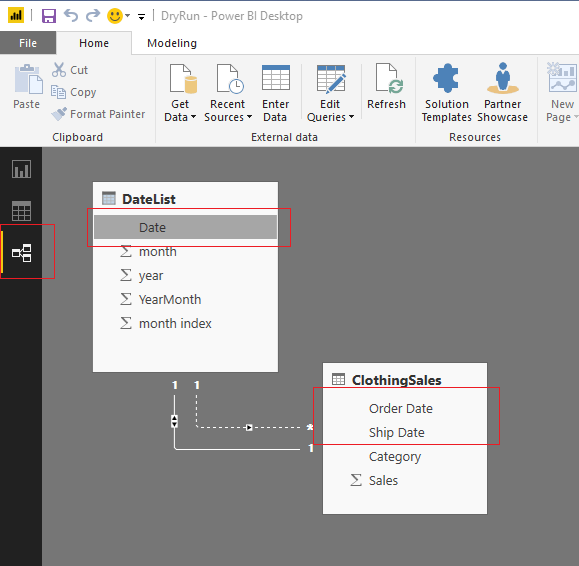
Linked Tables
By default, Power BI will only allow one active connection between tables. Therefore, we have one connection active and the other has been inactivated by default. Return to the report view by clicking the Report icon on the left black navigation bar.
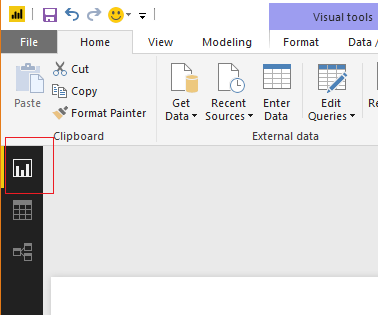
Report View
Now that we have completed the data modeling let’s make some visuals. We will start by making a simple table to see what the data is doing. Add the columns from the two tables, ClothingSales and DateList to a Table Visual.
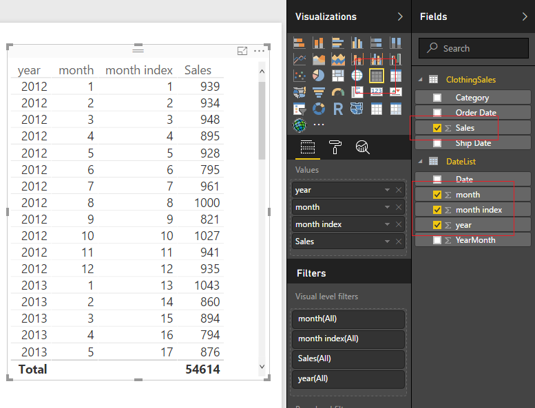
Create Table Visualization
Great! Now we have the total number of sales based on the order date. We know this because it is the primary connection that we established earlier when we linked our two tables together. But, what if I wanted to know the sales that were shipped based on the Ship Date. Earlier we made this connection but it is inactive.
Here is the awesomeness! We can create a measure that calculates different results between a user specified relationship.
First, we will re-calculate the sales number that we already have in our table. On the Home ribbon click the New Measure and enter the following in the DAX formula bar:
Order Date Sales = CALCULATE ( SUM ( ClothingSales[Sales] ), USERELATIONSHIP ( ‘DateList ‘[Date], ClothingSales[Order Date] ) )
Note: In this DAX formula we are creating a explicit measure, meaning we are specifically telling Power BI to sum a column. An implicit calculation is what we did earlier when we added the sales column to the table.
The USERELATIONSHIP filter within the calculation forces Power BI to calculate the sum based on the dates listed in the Order Date column. To see another demo on UseRelationship you can watch this video from Curbal.
Create another measure with the following DAX formula:
Ship Date Sales = CALCULATE ( SUM ( ClothingSales[Sales] ), USERELATIONSHIP ( ‘DateList ‘[Date], ClothingSales[Ship Date] ) )
This time we are forcing Power BI to use the inactive relationship to calculate the sum of the sales by shipped date. Add the two new measures to our table and we now can see how the calculations differ.
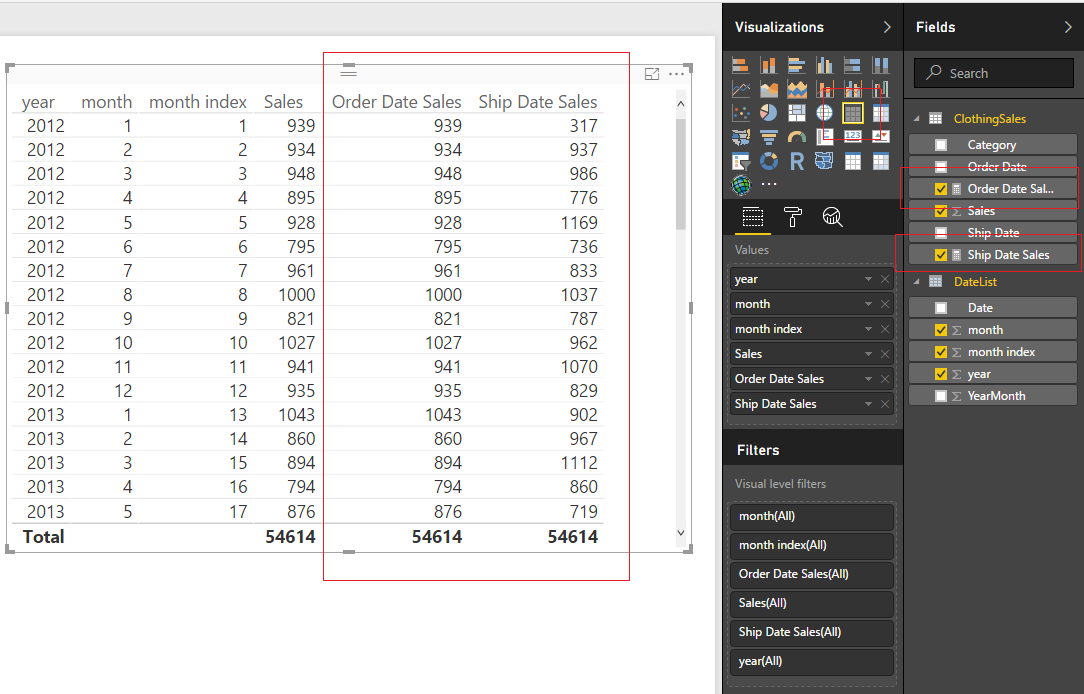
Sales By Order & Ship Date
The calculated sales for the order dates match our earlier column. This is expected, and we can confirm that this calculation is working properly. The shipped date sales are now calculating a different number. In some cases, the Shipped Date Sales is lower than the orders, because in that month you took in more orders than you shipped. In other months, the Shipped Date Sales is higher than the Order Date Sales, because there were likely large shipments ordered in the prior month and shipped in a different month.
By adding a Bar Chart from the Visualizations pane, we can now see sales by order date and ship date.
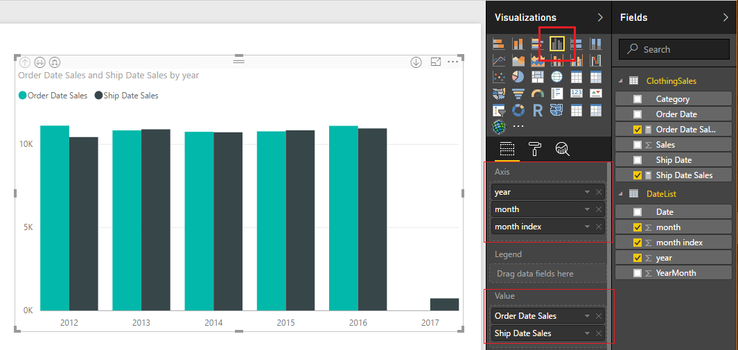
Bar Chart by Year
We can even dig deeper into the data. Click the Expand button to see the data by Year and Month.
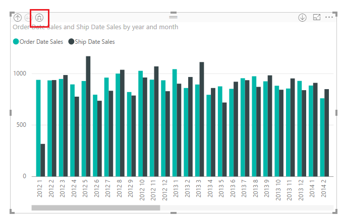
Expand Button
Well that is about it. I hope you enjoyed this tutorial about using two relationships between data tables. If you want more information about DAX check out these books that I have found extremely helpful.
This specific example was based of the article from Marco Russo at SQLBI on UserRelationship in Calculated Columns. Follow Marco at http://www.sqlbi.com/articles/
