Year: 2016

  • Santa Loves Power BI and R

    Santa Loves Power BI and R

    This past week I was talking with the big guy up north, jolly old fella, and the discussion came up about his toy production levels.  Santa was complaining about how hard it was to measure the performance of all his elves.  Naturally I started babbling about how much I enjoy Power BI and that I use it on all kinds of sources of data, google analytics, excel sheets, sharepoint, and SQL data warehouses just to name a few.  Now by this point most people would have wandered off looking for another conversation, but I must have struck a chord with Santa.  He jumped right in the conversation and told me how he had just moved all his local data centers into Azure and more specifically SQL data warehouses.  It was saving him loads of money in addition it has freed up all his I.T. elves to move to more important tasks, building the NES Classic for Nintendo, they are way behind in production.  To make a long story longer, I was able to convince Santa to give me a small sample of data so I could show him how to use R to visualize his data in PowerBI.  Here is what I came up with:
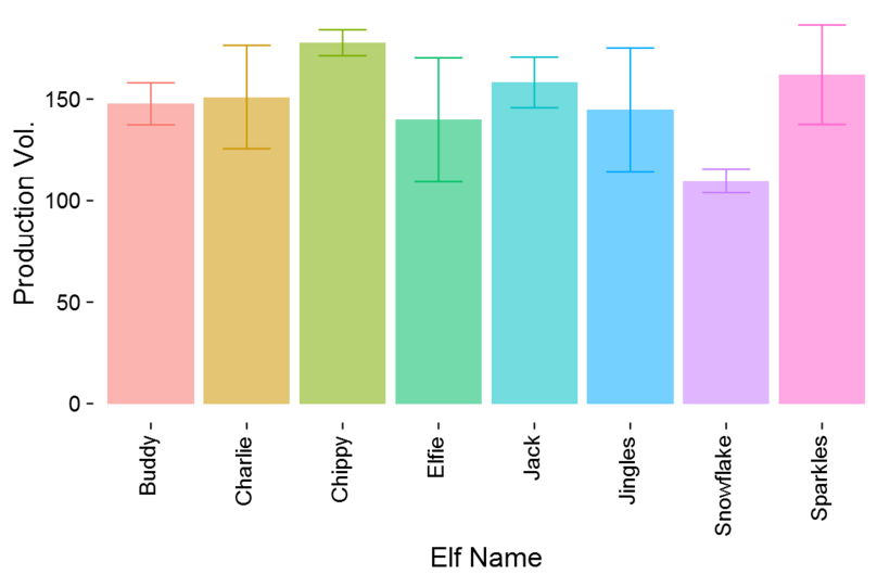
    Santa Production Levels
    Santa Production Levels

    Needless to say he was very pleased.  I explained the chart to Santa, each bar represents the average production volume for each elf.  Then the whiskers at the end of the bar represent the +1 and -1 standard deviation away from that mean.  It essentially tells you how consistent each elf is able to produce products and what is the average production rate.  For example, Buddy the Elf can produce an average 148 items in a day, he has a daily variance of 10 items.  Charlie can produce on average more items but has a wider daily variance.  Snowflake has the lowest average production level but is one of the more consistent producers.  Santa gave me a big smile and said “nice job.”

    Let’s walk through how I did this.

    Open up PowerBI Desktop, Click the Get Data button on the Home ribbon and select Blank Query.  Click Connect to open the Query Editor.  Click Advanced Editor on the View ribbon.  While in the Advanced Editor paste the following code into the editor window, click Done to complete the data load.

    Note: If you need some more help loading the data follow this tutorial about loading data using the Advanced Query Editor.  This tutorial teaches you how to copy and paste M code into the Advanced Editor.

    let
        Source = Excel.Workbook(Web.Contents("https://powerbitips03.blob.core.windows.net/blobpowerbitips03/wp-content/uploads/2016/12/Santa-Production.xlsx"), null, true),
        Production_Table = Source{[Item="Production",Kind="Table"]}[Data],
        #"Changed Type" = Table.TransformColumnTypes(Production_Table,{{"Elf", type text}, {"Toy", type text}, {"Prodution Volume", Int64.Type}})
    in
        #"Changed Type"

    Before you exit the query editor Rename the query to Production. It should look similar to the following:
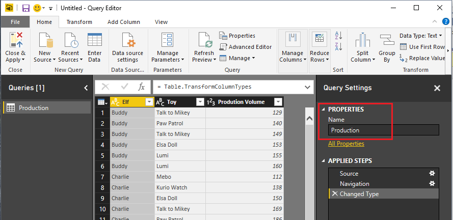
    Production Query
    Production Query

    Click Close & Apply on the home ribbon.

    Add the following measures by click on the New Measure button on the Home ribbon.

    Avg = AVERAGE(Production[Prodution Volume])

    The Avg measure will determine the height of each bar in the bar chart.

    StdDev = STDEV.P('Production'[Prodution Volume])

    The StdDev will calculate the standard deviation for each elf.

    Ymax = [Avg]+ [StdDev]

    The Ymax calculation adds the Avg measure value to the standard deviation for production.  This produces the upper arm of the whisker.

    Ymin = [Avg]-[StdDev]

    The Ymin calculation is subtracts the standard deviation from the Avg measure value.  This produces the lower arm of the whisker.

    Once you have completed making all the measures you should have a Production table with the following fields:
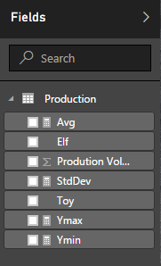
    Added Measures
    Added Measures

    Add the table visual by click on the Table visual in the Visualizations pane.  Add the Fields which are shown below.  Your table should look identical to this:
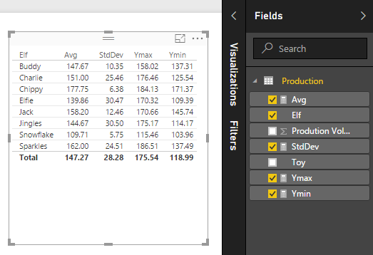
    Production Table
    Production Table

    Next, add the R Visual from the visualization Pane.  When you click on this you will get a message stating “Enable Script Visuals” click Enable to proceed.

    Note: If you have not installed R or enabled the preview features of R in Power BI you should follow this tutorial which helps you get everything set up.  For this particular visual we are using ggplot2.  This is a package for R and should be installed in the R environment.  You can follow this tutorial on how to install ggplot2.

    Add the following fields into the R visual:
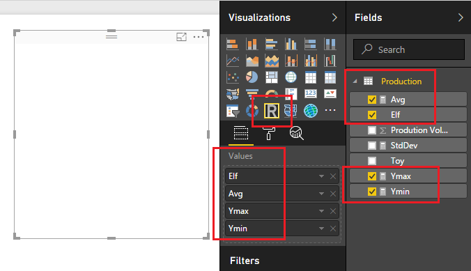
    Add Fields to R Visual
    Add Fields to R Visual

    Next in the R Script Editor add the following code to generate the R Script.

    library (ggplot2) # Load ggplot to run visuals

    # Set up graph
    ggplot(dataset, aes(x = Elf, y = Avg) ) +

    # Insert the bar chart using acutal values passed to visual
    # Stat = “identity” does not count items uses actual values
    # set up transparency to 70% with Alpha
    geom_bar( stat = “identity”, aes( alpha= 0.7, fill = Elf ) ) +
    # draw the error bars, use pass Ymin & Ymax from PBI
    geom_errorbar(aes(width = .5, colour = Elf , ymin = Ymin, ymax = Ymax)) +

    # Change the Labels
    labs(x = “Elf Name”, y = “Production Vol.” ) +

    # Make the theme simple and remove gridlines
    # Change the font size to 14
    theme_classic( base_size = 18 ) +

    # Remove the legend
    theme( legend.position = “none”) +

    # Change elements of the Axis, Angle, horizontal & Vertical position
    theme( axis.text.x = element_text(angle = 90, hjust = 1, vjust = 0.3),
    axis.text = element_text(colour = “black”),
    axis.ticks = element_line(colour = “black”),
    axis.title = element_text(colour = “black”),
    plot.background = element_rect(colour = NA) )

    Note: This code uses the R package ggplot2.  It will error out if you don’t have ggplot2 installed. 

    Click the run icon to execute the R script.
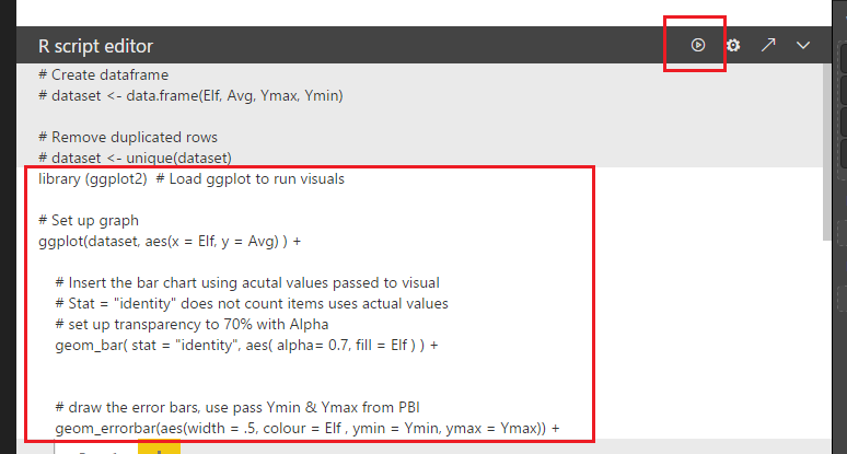
    Add R Script
    Add R Script & Run Script

    When the script runs you will have a beautiful production chart.
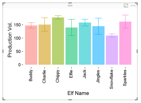
    R Chart
    R Chart

    Thanks for following along.  Like always be sure to share if you liked this content.  I am always, looking for feedback and possible topics so make sure you leave a comment below.

    If you want to download a similar example already completed you can download this example from the R Script Showcase (don’t forget to give me a thumbs up).

    Merry Christmas!

  • Measures – Year Over Year Percent Change

    Measures – Year Over Year Percent Change

    This tutorial is a variation on the month to month percent change tutorial.  This specific exploration in year over year performance was born out of reviewing my google analytics information.  The specific analysis question I am trying to answer is, how did this current month of website visitors compare to the same month last year.  For example I want to compare the number of visitors for November 2016 to November 2015.  Did I have more users this year in this month or last year?  What was my percent changed between the two months?

    Here is a sample of the analysis:

    let’s begin with loading our data and data transformations.  Open up PowerBI Desktop, Click the Get Data button on the Home ribbon and select Blank Query.  Click Connect to open the Query Editor.  Click Advanced Editor on the View ribbon.  While in the Advanced Editor paste the following code into the editor window, click Done to complete the data load.

    Note: If you need some more help loading the data follow this tutorial about loading data using the Advanced Query Editor.  This tutorial teaches you how to copy and paste M code into the Advanced Editor.

    let
     Source = Table.FromRows(Json.Document(Binary.Decompress(Binary.FromText("VdDBDcQwCETRXnyOFMAYcC1W+m9jV8BhfH1ygJ9zBr/8CvEaz+DYNL7nDAFjnWkTTNsUbIqnLfyWa56BOXOagy2xtMB5Vjs2mPFOYwIkikIsWd6IKb7qxH5o+bBNwIwIk622OCanTd2YXPNUMNnqFwomp0XvDTAPw+Q2uZL7QL+SC1Wv5Dpx/lO+Hw==", BinaryEncoding.Base64), Compression.Deflate)), let _t = ((type text) meta [Serialized.Text = true]) in type table [#"Start of Month" = _t, Sales = _t]),
     #"Changed Type" = Table.TransformColumnTypes(Source,{{"Start of Month", type date}, {"Sales", Int64.Type}}),
     #"Inserted Month" = Table.AddColumn(#"Changed Type", "Month", each Date.Month([Start of Month]), type number),
     #"Inserted Year" = Table.AddColumn(#"Inserted Month", "Year", each Date.Year([Start of Month]), type number)
    in
     #"Inserted Year"

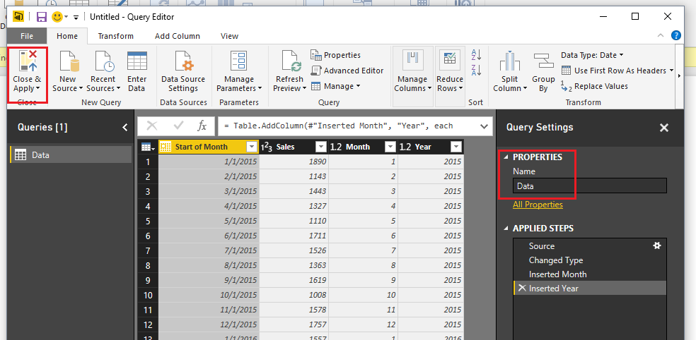
    While still in the Query Editor rename the query to Data.  Then click Close & Apply to complete the data load into the data model.

    Load Monthly Data
    Load Monthly Data

    Next, make four measures.  On the Home ribbon click the New Measure button.  Enter the following to establish a reference date to the subsequent equations:

    Date Reference = DATE(2016,12,31)

    Enter in the following equation to calculate the last year monthly sales amount.

    LastYear = 
      VAR 
        CurrentDate = [Date Reference]
      RETURN
        CALCULATE( 
         SUM(Data[Sales]), 
         Data[Year] = YEAR(CurrentDate)-1
        )

    Note: Using the NOW() function calls the current time when the query was last run.  Thus, if you refresh your data next month the NOW() function wrapped in a YEAR() will return the current year from the date-time observed by PowerBI.

    Following the same process enter the following additional measures.  The ThisYear measure calculates the sales for the current month.

    ThisYear = 
      VAR 
       CurrentDate = [Date Reference] 
      RETURN
       CALCULATE(SUM(Data[Sales]),Data[Year] = YEAR(CurrentDate))

    Finally, add the calculation for the Year to Year comparison.

    YoY Percent Change = DIVIDE([ThisYear], [LastYear], 0)-1

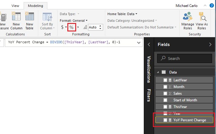
    Since the YoY Percent Change is a real percentage we need to change the formatting to a percent.  Click on the YoY Percent Change measure then on the Modeling ribbon click the symbol in the formatting section of the ribbon.

    Change Measure Format
    Change Measure Format

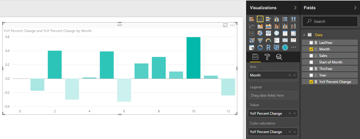
    Next, add a Stacked Column Chart with the following columns selected.

    Add Stacked Column Chart
    Add Stacked Column Chart

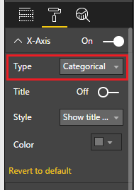
    OK, we have a chart, but it is kinda awkward looking right now.  The x-axis is the month number but we don’t have a month 0.  That simply does not make sense.  Let’s change some of the chart properties.  While having the Stacked Column Chart selected click on the Paint Roller in the Visualizations pane.  First, click on the X-Axis and change the Type to Categorical.

    Change X-Axis
    Change X-Axis

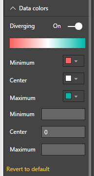
    Then click on the Data Colors and turn on Diverging.  Change the Minimum color to Red and the Maximum color to Green.  Set the Center to a value of 0.

    Change Colors
    Change Colors

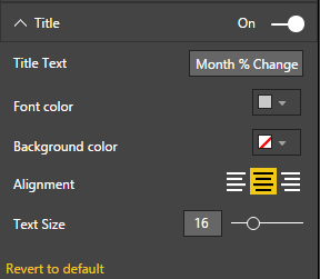
    Click on the Title change it something meaningful, Center the text and increase the font size.

    Change Title
    Change Title

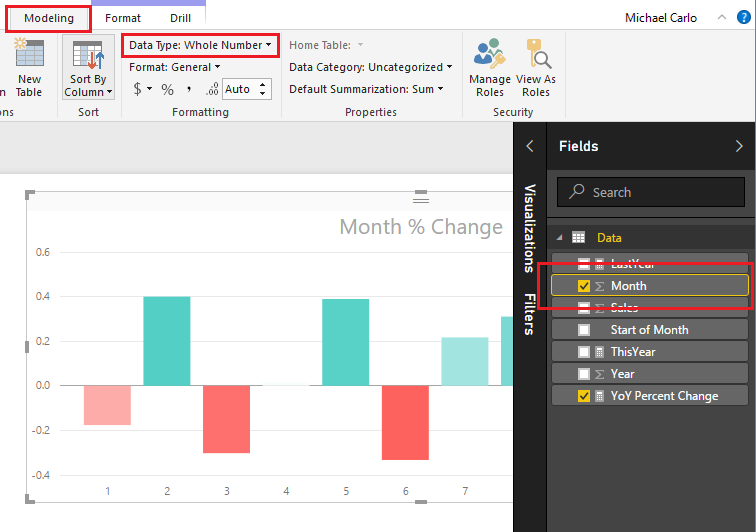
    Our bar chart looks much better.  However, the month numbers do not look quite right.  Visually the month indicators would be cleaner if we didn’t have any decimals.  Click on the Month field and then on the Modeling ribbon change the Data Type to Whole Number.  There will be a warning letting you know that you are changing the Data Type of the Whole number.  Click OK to proceed with the change.

    Change Month to Whole Number
    Change Month to Whole Number

    Another successful percent change tutorial completed.  I hope you enjoyed this year over year month comparison example.  Make sure you share if you like what you see.

  • Grouping and Improved Date Slicer

    Grouping and Improved Date Slicer

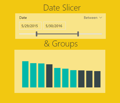
    In the October update of PowerBI Desktop we were given a number of really useful features, ranging from a new Date Slicer, Grid lines, Grouping, Binning, Top N Filters, and R-powered custom visuals.  For the full release on the October 2016 software release you can read more here.

    For those of you who have followed my site you already know that I absolutely love the ability to create R-visuals within PowerBI.  If you want to learn more you can read the R script tutorials here.

    As I’ve been exploring this October release of Power BI Desktop two features have really stood out.  First, the ability to use the Date Slicer and second the new feature of Grouping for Bar Charts.  In my daily work flow I have struggled in the past with solutions which are now solved.

    Welcome to my love & hate relationship with time bound data sets.  Inevitability at some point you will encounter a need to manipulate data over time.  Common business questions will come in the form of:  What was my percent change compared from this month compared to last month?  What is my sales performance for this year? Are we up or down compared to the same period last year?  While these questions are simple I have found that calculating measures and subsequently building visuals can get very complex in a hurry.  Enter the Date Slicer.  Let me be clear, the Date Slicer will not solve all your problems, it does present a very useful interface that will let report users quickly navigate through their time delineated data.

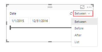
    What is the Date Slicer?  I’m glad you asked. Behold….

    Date Slicer
    Date Slicer

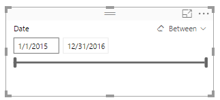
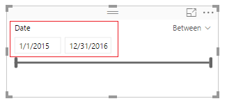
    Here are a couple of key items to point out.  On the left side of the visual you are given the ability to select the starting date, and ending date.

    Start and End Dates
    Start and End Dates

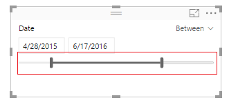
    The bottom of the Date Slicer has an adjustable time bar that allows quick time adjustments.

    Changed Timeline
    Changed Timeline

    On the right side of the visual you can toggle between different date selection modes, Between, Before, After, and List.

    Time Parameter Selector
    Time Parameter Selector

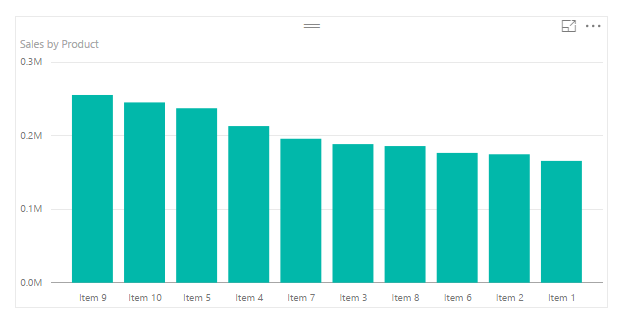
    Ok, enough about the Date Slicer, how about the Groupings feature.  Lets say you start off with a bar chart that looks similar to the following:

    Sample Bar Chart
    Sample Bar Chart

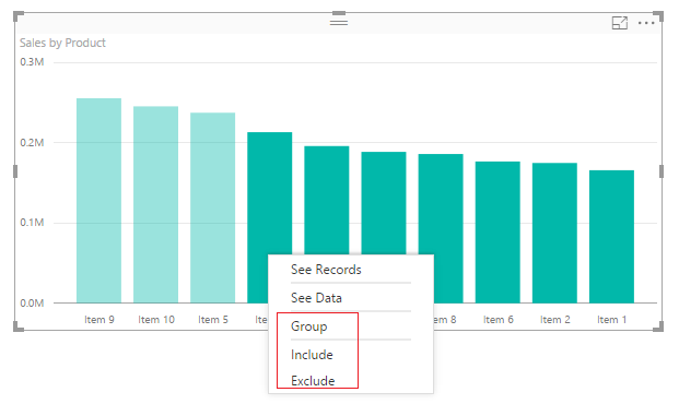
    Well, maybe you’re only interested in Items 9, 10, and 5.  Grouping now allows the selection of multiple bars and by right clicking you can Group, Include, or Exclude.

    Right Click on Selected Data Bars
    Right Click on Selected Data Bars

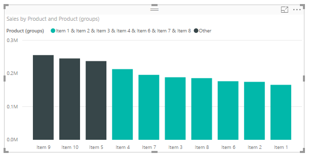
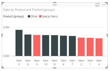
    Clicking group creates a new column in the Fields area that groups the items together and adds them to the chart legend.

    Grouped Items in Bar Chart
    Grouped Items in Bar Chart

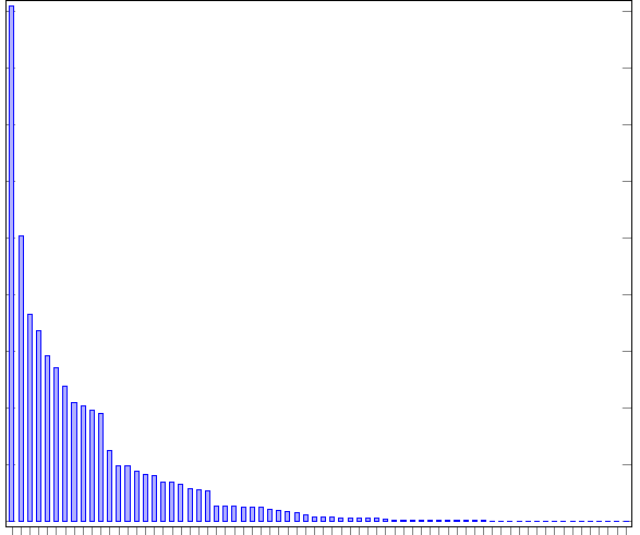
    Let me tell you this is helpful, especially when your bar chart looks like this:

    Ugly Bar Chart
    Ugly Bar Chart

    Be honest, you have published a report or two when there were just way to many bars.  The different between the largest bar and all the small bars barely tells you any information.  This is why grouping is helpful.  When you receive data and you need to focus your story to the important pieces then grouping is your friend.

    Enough babbling, let’s get to the tutorial.

    Open up PowerBI Desktop, Click the Get Data button on the Home ribbon and select Blank Query.  Click Connect to open the Query Editor.  Click Advanced Editor on the View ribbon.  While in the Advanced Editor paste the following code into the editor window, click Done to complete the data load.

    Note: If you need some more help loading the data follow this tutorial about loading data using the Advanced Query Editor.  This tutorial teaches you how to copy and paste M code into the Advanced Editor.

    let
     Source = Excel.Workbook(Web.Contents("https://powerbitips03.blob.core.windows.net/blobpowerbitips03/wp-content/uploads/2016/11/Sales-Data-Two-Years.xlsx"), null, true),
     Sales_Table = Source{[Item="Sales",Kind="Table"]}[Data],
     #"Changed Type" = Table.TransformColumnTypes(Sales_Table,{{"Date", type date}, {"Product", type text}, {"Sales", Int64.Type}})
    in
     #"Changed Type"

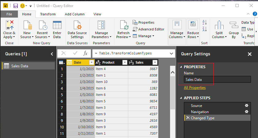
    Rename the Query to Sales Data.  Once you’ve completed the data load your data should look like the following.

    Load Sales Data
    Load Sales Data

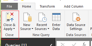
    On the Home ribbon click Close & Apply to complete the data load.

    Close and Apply
    Close and Apply

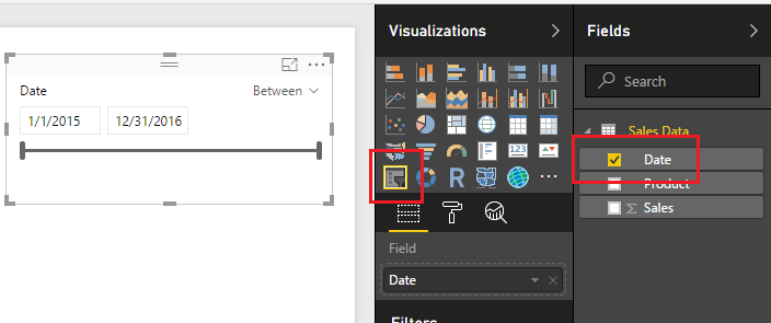
    Great, we are ready to start adding visuals now.  Add a Slicer visual from the Visualizations window and populate the visual with the Date field.  By default, the slicer will auto recognize that the field being added is a date and will automatically show the Date Slicer.

    Add Date Slicer
    Add Date Slicer

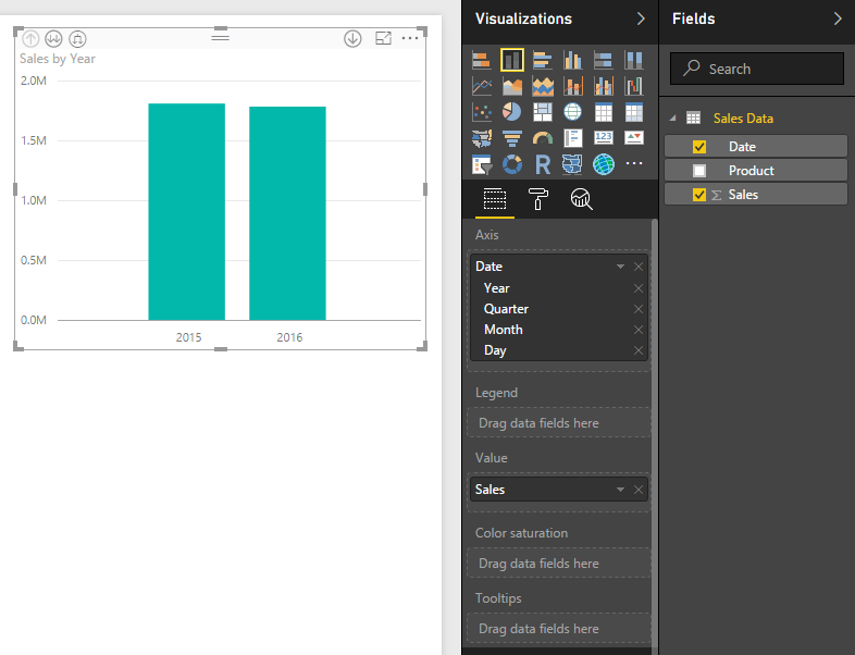
    Next, add a bar chart visualization.  The Date field will be the Axis, and the Sales will be the Value.

    Add Bar Chart
    Add Bar Chart

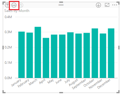
    Again by default the Date filed will be entered as a Hierarchy field.  Click the Drill Down button until you see a monthly view of the date.  This should require two clicks, the first drills down to quarters, then second click drills down to month level.  After doing this your visual should look like the following:

    Drill Down to Month
    Drill Down to Month

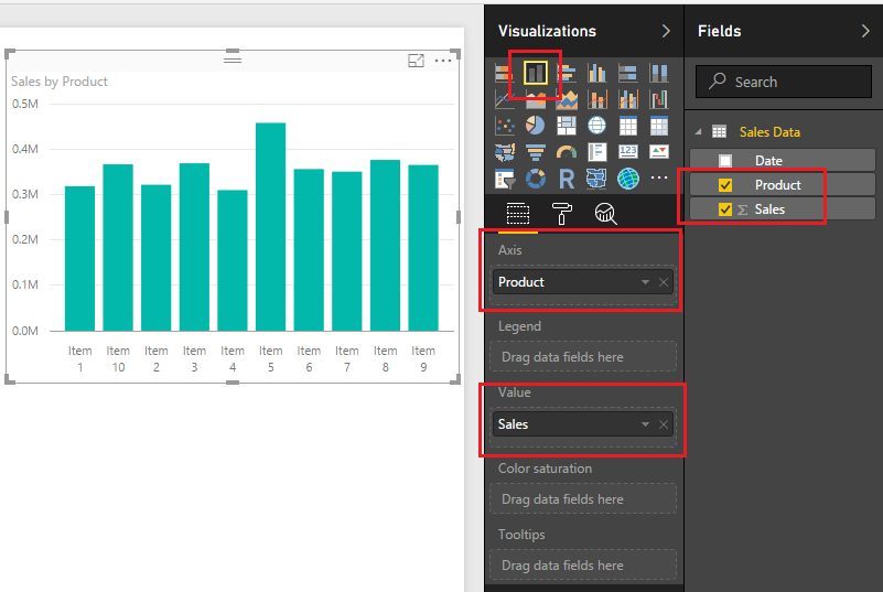
    Add a second bar chart with following fields selected.

    Second Bar Chart
    Second Bar Chart

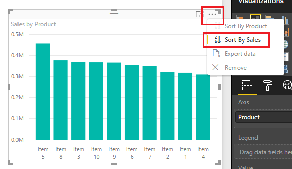
    Sort the Sales by Product bar chart in descending sale order by clicking the Ellipsis and when the drown down menu appears selecting Sort by Sales.

    Descending Sort by Sales
    Descending Sort by Sales

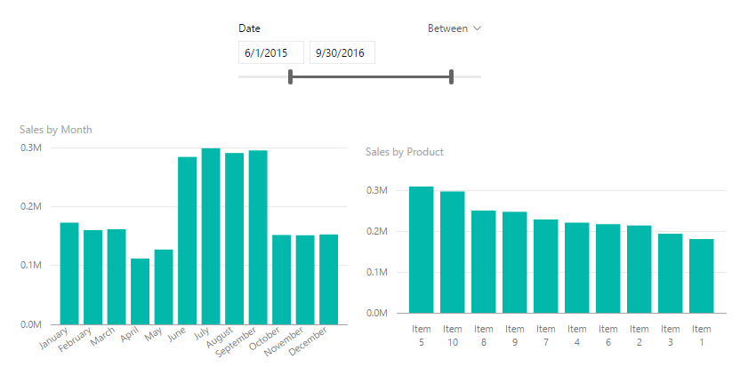
    Now that we have built a couple visuals and a Date Slicer, take some time to explore how the Date Slicer interacts with the bar charts.  In the example below I modified the starting date to 6/1/205 and the ending date to be 9/30/2015.

    Modify Date Slicer Properties
    Modify Date Slicer Properties

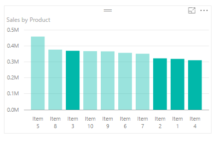
    To utilize the grouping feature we will group Items 1,2,3 and 4 together.  While holding the control button click Items 1,2,3 and 4 on the Sales by Product bar chart.

    Ctrl Click Items
    Ctrl Click Items

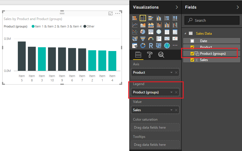
    Right click Item 3 an menu will appear, select Group.  Notice once you do this a new Product (Group) field appears in the field menu and the Product (Group) is automatically added to the legend of the bar chart visual.

    Grouping in Bar Chart
    Grouping in Bar Chart

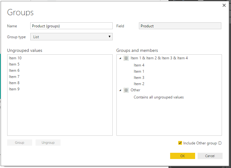
    To edit the grouping you can click on the Field labeled Product (groups) and select Edit Groups.  Doing this reveals the grouping dialog box.

    Grouping Dialog Box
    Grouping Dialog Box

    You can rename the created group by double clicking the name Item 1 & Item 2 & Item 3 & Item 4.  

    Rename Grouping
    Rename Grouping

    Change the name of the grouping to be titled Special Items.  Click OK to close the Groups dialog box. Notice how the bar chart updates the legend values to renamed grouping.

    Rename Group
    Rename Group

    Well, that wraps up this tutorial.  I hope you enjoyed it.  Below is a live demo of what we built today.

    Make sure you share the content if you liked this tutorial.

  • Pareto Charting in PowerBI

    Pareto Charting in PowerBI

    The Pareto chart is a handy visual, but is not so easy to build in either excel or PowerBI.  In a Pareto chart, information is provided about an individual product or category as a bar, and a cumulative scale as a line which compairs all bars.  This type of visual can be extremely helpful when conducting failure mode analysis, causes of a problem, or even product portfolio balances.  For some more information on Pareto charts you can learn more here or here.  If you’re interested in building a Pareto chart in excel, I have found this post from Excel Easy to be helpful.

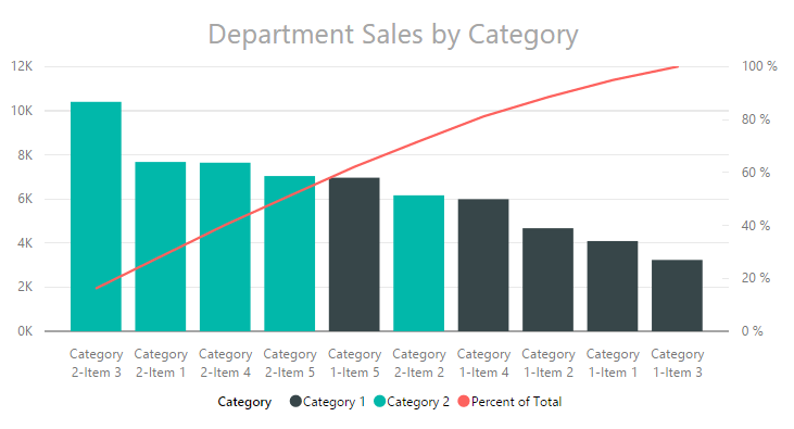
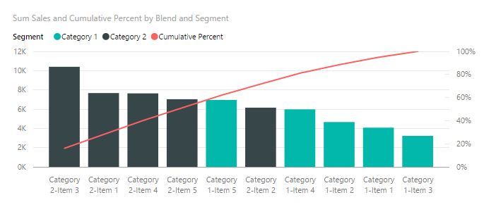
    To give you a little teaser of what we will be building today, below you will see an image of the final Pareto chart.  On the left side we have sales of units, and on the right is the cumulative percent of all sales.  Using the Pareto chart a user has the ability to see which products comprise the majority of your sales.  For example, the first 4 bars total approximately 50% of all sales.

    Pareto Final Product
    Pareto Final Product

    Alright, let’s get started.

    Open up PowerBI Desktop, Click the Get Data button on the Home ribbon and select Blank Query.  Click Connect to open the Query Editor.  Click Advanced Editor on the View ribbon.  While in the Advanced Editor paste the following code into the editor window.

    Note: If you need some more help loading the data follow this tutorial about loading data using the Advanced Query Editor.  This tutorial teaches you how to copy and paste M code into the Advanced Editor.

    let
     Source = Excel.Workbook(Web.Contents("https://powerbitips03.blob.core.windows.net/blobpowerbitips03/wp-content/uploads/2016/10/Sample-Data.xlsx"), null, true),
     Table1_Table = Source{[Item="Table1",Kind="Table"]}[Data],
     #"Changed Type" = Table.TransformColumnTypes(Table1_Table,{{"Item", type text}, {"Sales", Int64.Type}, {"Segment", type text}})
    in
     #"Changed Type"

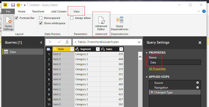
    Rename the Query to Data.  Once you’ve completed the data load your data should look like the following.

    Load Data to Query Editor
    Load Data to Query Editor

    On the Home ribbon click Close & Apply to complete the data load.

    Close and Apply
    Close and Apply

    Let’s begin with a little exploration of our data.

    Pro Tip: When I am building reports I often load the data and then immediately start building a couple of tables and slicers.  It helps me understand how my data reacts to the slicers and helps me determine how to shape the data so that the visuals will work properly.  For this example, we only have one table, but when loading data things can get rather complex due to loading multiple tables with multiple relationships.

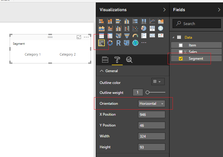
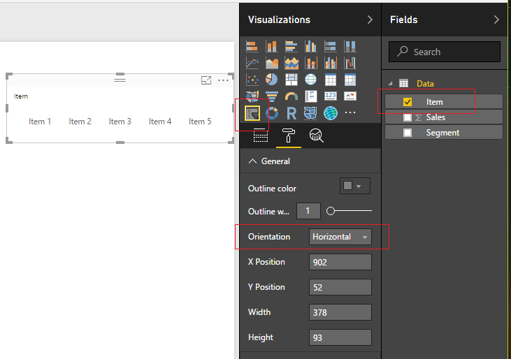
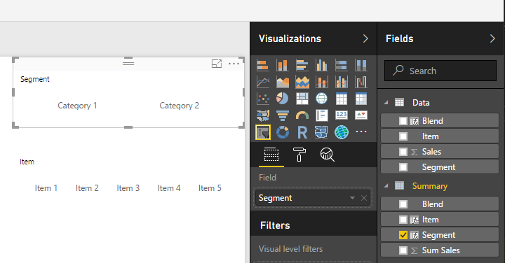
    Add a Slicer for the Segment.  Enhance the look of the slicer by changing it from a vertical to a horizontal slicer.  While the slicer is highlighted, click the Paint Roller expand the General section and change the orientation from vertical to Horizontal.

    Segment Slicer
    Segment Slicer

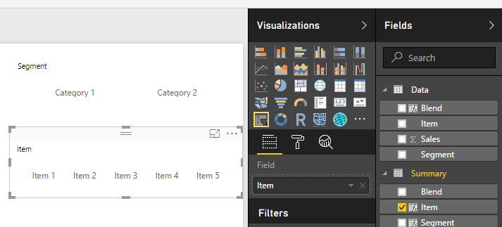
    Repeat the same process to add a Slicer for the item field.

    Item Slicer
    Item Slicer

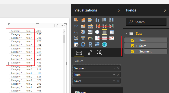
    Next, add a table view of all the fields.  Start with Segment, then Item and finally add Sales to the Table Visual.

    Data Table
    Data Table

    Notice, now that we added all the Fields, there are a number of repeating values.  We have Category 1 and Item 1 repeated 9 times.  In some cases, it will be necessary to have this level of data brought into the data model within PowerBI.  A common reason is that this level of granularity is required for other report pages, or visuals.  It is OK to bring large amounts of data, but as a method of best practice it is recommended that you bring in the data required to support the visuals.

    Now, to address these multiple items that we see in our data.  In the sample Pareto image provided at the beginning of this Tutorial we only had one bar for Category 2 Item 3.  Thus, we need to summarize each grouping of every Category and Item combination.  To do this we will construct a summary table.

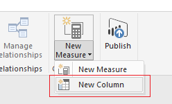
    First, we will create a unique Key that will be used to summarize each combination of Category and Item pair.  Click the bottom half of the New Measure button located on the Home ribbon.

    Calculated Column
    Calculated Column

    Enter the following DAX expression.  This new column titled Blend will be the unique Key that is utilized to summarize the data.

    Blend = Data[Segment]  &  "-"  &  Data[Item]

    Select the Modeling ribbon and then click on the New Table button.  Enter the following DAX expression.

    Summary = SUMMARIZE('Data', Data[Blend], "Sum Sales", SUM(Data[Sales]) )

    For more information on the SUMMARIZE function you can visit the Mircosoft Summarize documentation page.  In this equation we first select the table and in this case it is ‘Data’.  Then the column we want to summarize or group by is the Segment column noted as Data[Blend].  The next field is the title of the summarized field column, noted as “Sum Sales”.  Then DAX function that calculates the Sum of the column labeled Data[Sales], noted as SUM(Data[Sales]).  It is relevant to point out here that the SUMMARIZE function will only work with building a new table and not as a calculated column or measure.

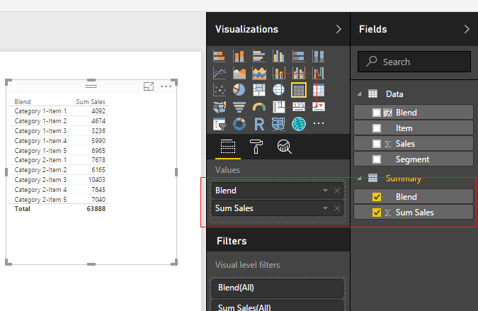
    Add a new Table visual to the report and include the two newly created fields from the Summary table.

    Summary Table Visual
    Summary Table Visual

    We have a field titled Blend which is our Key for all the summarized groupings.  Next, we will want to parse out the Segments and Items from this blend column.  We will want to use Category 1 & 2 in a slicer and the same for Items 1 to 5.  Highlight the summary table by clicking the grey space next to the word Summary.  Click the New Column button on the Modeling ribbon and enter the following DAX expression.

    Segment = PATHITEM(
       SUBSTITUTE(Summary[Blend], "-" , "|" ),
       1 )

    In this expression the Substitute function replaced the dash “-” with a “|” character.  Then the PATHITEM function can then parse the text into segments.  By entering a 1 we select the first item in the sequence.  For our example we only have two items, but when you’re working with file paths you can have multiple items in the path such as “\users\mike\my documents\my folder\”, which would equate to users = position 1, mike = position 2, my documents = position 3, etc..

    Add another new column with the following DAX expression for the item column.

    Item = PATHITEM( 
      SUBSTITUTE(Summary[Blend], "-" , "|" ),
      2 )

    Note: We changed the PATHITEM position from 1 to 2.

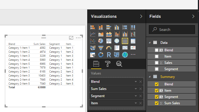
    Next add the newly created Segment and Item columns to our summary table visual that we created earlier.

    Add New Fields
    Add New Fields

    Nice job so far.  Now we have to modify our slicers to point to the new Item and Segment fields we created in the Summary table.  Select the Segment Slicer Visual and add the Segment Field from the Summary table.

    Update Segment Slicer
    Update Segment Slicer
    Update Item Slicer
    Update Item Slicer

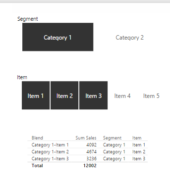
    Now that we have updated the slicers, we can now can control the table visual made from the Summary table.

    Select Category 1 and Items 1 to 3
    Select Category 1 and Items 1 to 3

    Pro Tip: To select multiple items in a slicer you can hold down the Ctrl button on the key board and click multiple slicer items.  This is how I was able to select Items 1 to 3.

    Now we are ready to build the measures that will support the Pareto chart.  Click on the bottom half of the New Measure button on the Home ribbon and select New Column.  Add the following DAX expression to rank all the items in the Summary table.

    Ranking = RANKX(  'Summary',   'Summary'[Sum Sales])

    Add a measure for the Cumulative total according to the new ranking column we created.  Click the top half of the New Measure button on the Home ribbon.  Add the following DAX expression.

    Cumulative Total = CALCULATE(
        SUM( Summary[Sum Sales] ),
        FILTER( ALLSELECTED( Summary ),
            Summary[Ranking] <= MAX( Summary[Ranking] )
        ))

    Repeat the add measure process and add a Total measure which will total only the items from the summary table that have been selected in the report view.  Add the following DAX expression.

    Total Sales = CALCULATE(
     SUM( Summary[Sum Sales] ) ,
     ALLSELECTED( Summary )
     )

    For the last measure, repeat the process to add another measure.  Enter the following DAX expression as a measure.

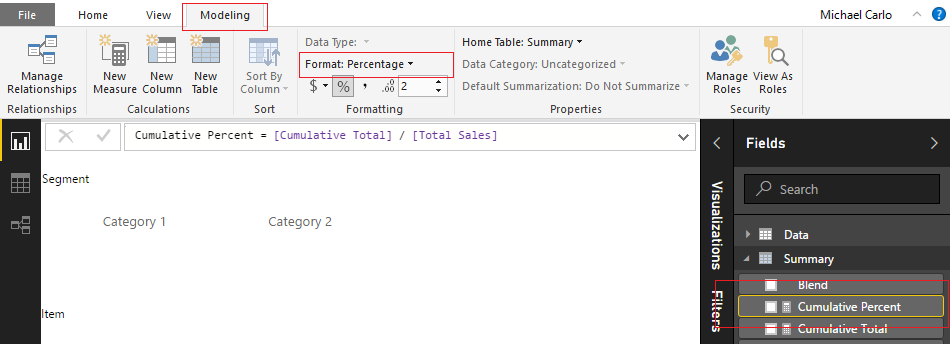
    Cumulative Percent = [Cumulative Total] / [Total Sales]

    The Cumulative Percent measure is a calculated as a percentage, thus we need to change this measure’s formatting to percentage.  Click the measure labeled Cumulative Percent then change the Format to Percentage which is found on the Modeling ribbon.

    Change Formatting
    Change Formatting

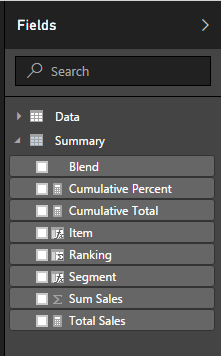
    Your Summary table should now look like the following.

    Updated Fields List
    Updated Fields List

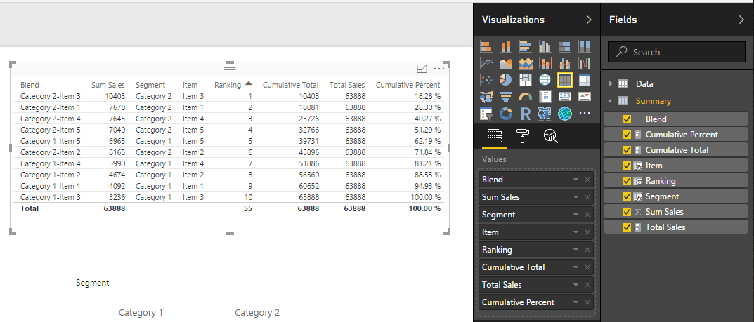
    To see all the calculations that we just created add all the fields from the Summary table to the Summary table visual we created earlier.

    Full Summary Table Visual
    Full Summary Table Visual

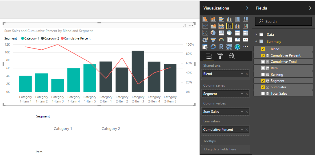
    At last, we are ready to add the Pareto chart.  Add the following fields to the line and stacked column chart.

    Add Line and Stacked Bar Chart
    Add Line and Stacked Bar Chart

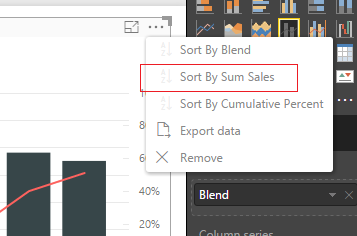
    Order the data in descending order by the number of sales by click the visual’s Ellipsis and selecting Sort By Sum Sales.

    Sort by Sales
    Sort by Sales

    This changes the order of the items to make a Pareto chart.

    Final Pareto Chart
    Final Pareto Chart

    Thanks for following along.  Share if you enjoyed this tutorial.

  • Map with Data Labels in R

    Map with Data Labels in R

    Mapping is one of the better features of PowerBI.  It is one of the more distinguishing feature differences between Excel and PowerBI.  You can produce a map inside an excel document using Bing maps, however, the experience has always felt a little like an after-thought.  Mapping within PowerBI has a planned, and thoughtful integration.  While the mapping functionalities within PowerBI Desktop are far improved when compared to excel, there are still some limitations to the mapping visuals.  This past week I encountered such an example.  We wanted to draw a map of the United States, add state name labels and some dimensional property like year over year percent change.

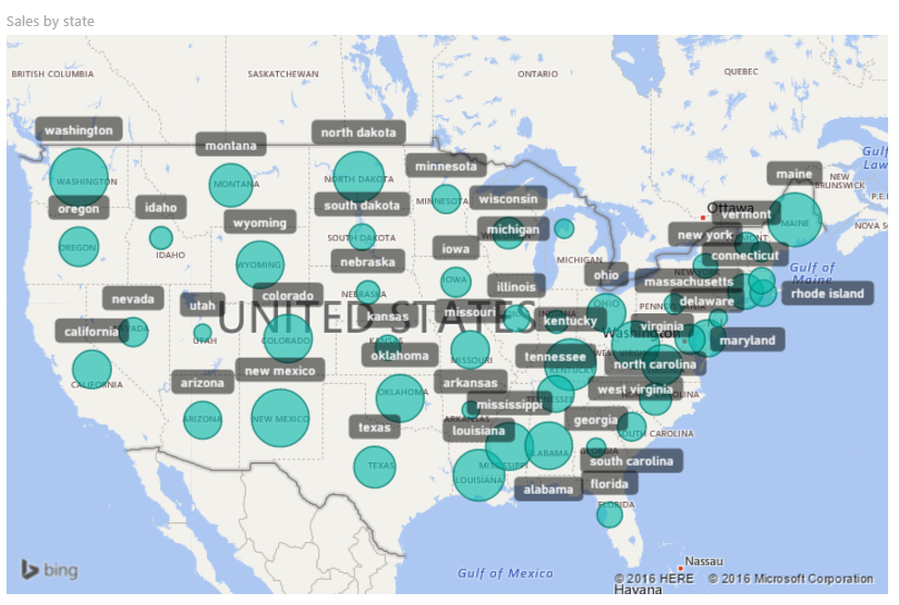
    I started with the standard map visual, but this didn’t work because there is no ability to shade each state individually.  This just looked like a bubbled mess.

    Globe Map Visual
    Globe Map Visual

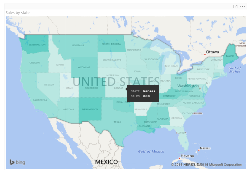
    Next, I tried the Filled Map visual.  While this mapping visual provides the colored states it lacks the ability to add data labels onto the map.  Clicking on the map would filter down to the selected state, which could show a numerical value.  Alternatively, you can place your mouse over a state and the resulting tag will show the details of the state (hovering example provided below).

    Filled Map Visual
    Filled Map Visual

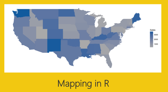
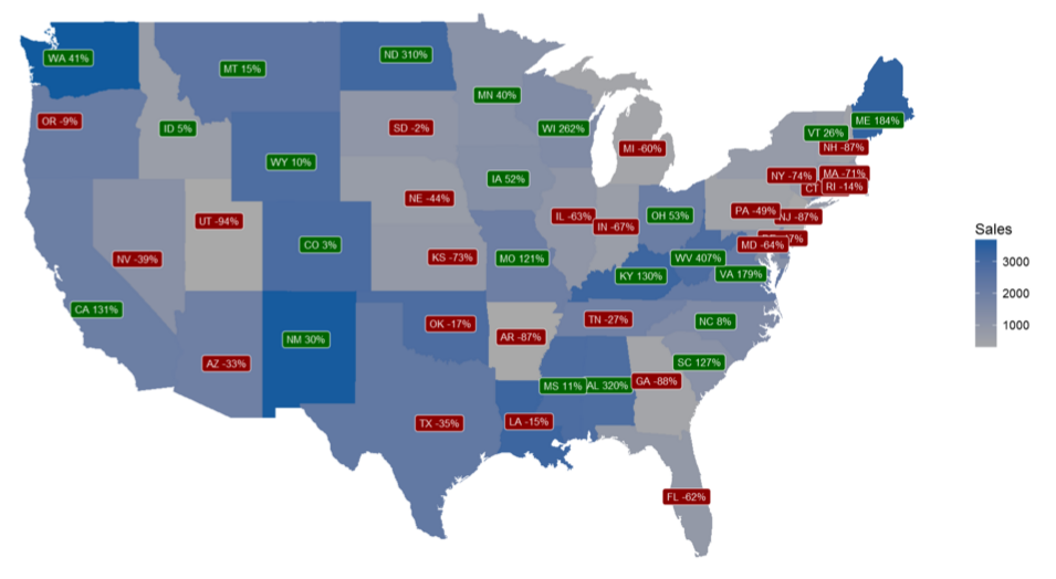
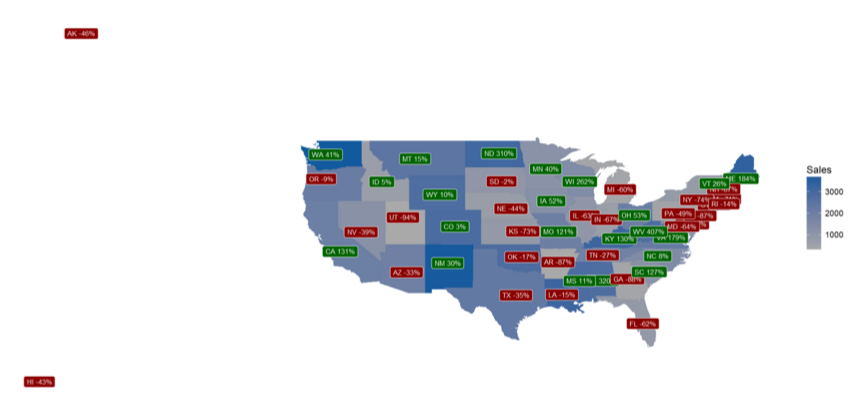
    Still this did not quite meet my visual requirements.  I finally decided to build the visual in R which provided the correct amount of flexibility. See below for final result.  You can download the pbix file from the Microsoft R Script Showcase.

    R Map Visual
    R Map Visual

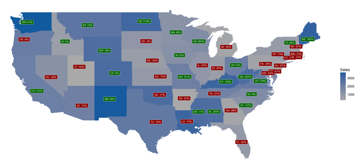
    In this visual, each state is shaded with a gradient color scale.  The states with the lowest sales are grey and the states with higher sales numbers transition to dark blue.  The darker the blue the more sales the state saw.  Each state has an applied label.  The color of the label denotes the percent change in sales.  If the color is green then the sales this year were higher than last year, red means that the state sales were lower this year.  The state name is listed in the label as well as the calculation for the year over year percent change.

    Alright, let’s start the tutorial.

    First, before we open PowerBI we need to load the appropriate packages for R.  For this visual you will need to load both the maps and the ggplot2 packages from Microsoft R Open.

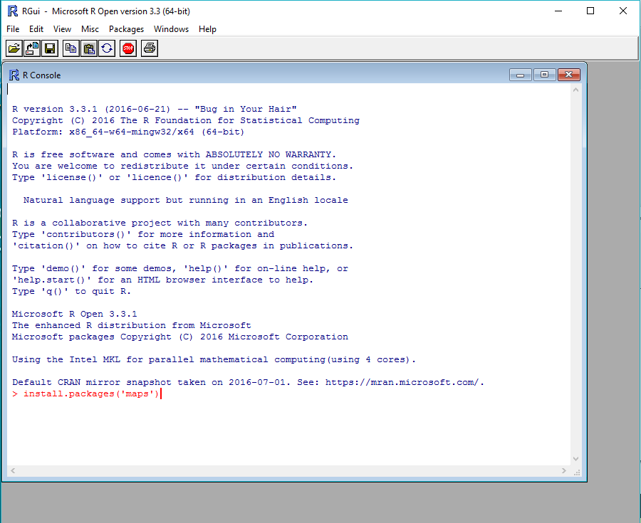
    Open the R console and use the following code to install maps.

    install.packages('maps')
    Install Maps Package
    Install Maps Package

    Repeat this process for installing ggplot2.

    install.packages('ggplot2')

    After installing the R packages we are ready to work in PowerBI Desktop.  First, we need to load our sample data.  Open up PowerBI Desktop and start a blank query.  On the View ribbon in the query editor open the Advanced Editor and enter the following M code.

    Note: If you need some more help loading the data follow this tutorial about loading data using the Advanced Query Editor.  This tutorial teaches you how to copy and paste M code into the Advanced Editor.

    let
      Source = Excel.Workbook(Web.Contents("https://powerbitips03.blob.core.windows.net/blobpowerbitips03/wp-content/uploads/2016/10/State-Data.xlsx"), null, true),
      StateData_Table = Source{[Item="StateData",Kind="Table"]}[Data],
      #"Changed Type" = Table.TransformColumnTypes(StateData_Table,{{"StateName", type text}, {"Abb", type text}, {"TY Sales", Int64.Type}, {"state", type text}, {"Latitude", type number}, {"Longitude", type number}, {"LY Sales", Int64.Type}, {"Chng", type number}}),
      #"Renamed Columns" = Table.RenameColumns(#"Changed Type",{{"TY Sales", "Sales"}})
    in
      #"Renamed Columns"

    After pasting the code into the Advanced Editor click Done to load the data.  While in the Query Editor, rename the query to be StateData, then click Close & Apply on the Home ribbon.

    Load Mapping Data
    Load Mapping Data

    We still need to prepare the data further by adding two calculated columns.  Click the bottom half of the New Measure button on the Home ribbon and select New Column.

    Add New Column
    Add New Column

    Enter the following code into the formula bar that appears after clicking New Column.

    Change = StateData[Abb] & " " & ROUND(100*StateData[Chng],0) & "%"
    Change Column Measure
    Change Column Measure

    Again, click on the New Column button found on the Home ribbon and add the code for a color column.

    Color = if(StateData[Chng] > 0 , "Dark Green", "Dark Red")
    Color Column Measure
    Color Column Measure

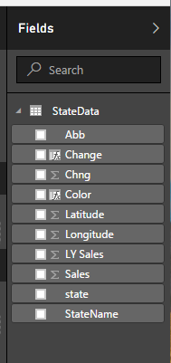
    The Fields list should now look like the following.

    Fields List
    Fields List

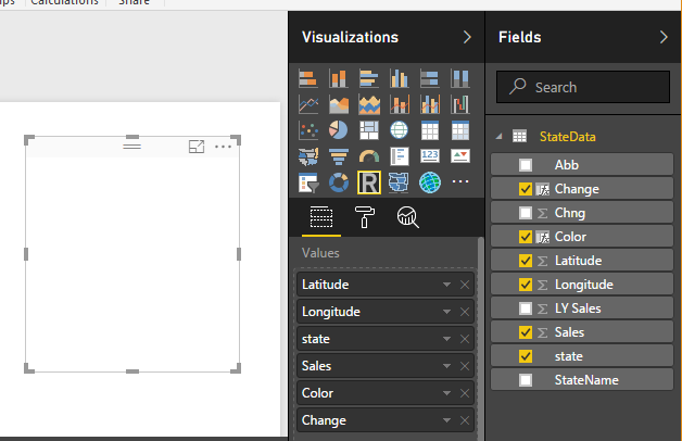
    Add the R visual with the following fields.

    R Visual Fields
    R Visual Fields

    Add the following R script into the R Script Editor.

    # Load the ggplot2 and maps packages
     library(ggplot2)
     library(maps)
    
    # Load the mapping data into a dataframe called states_map
     states_map <- map_data("state")
    
    # Start ggplot2 by sending it the dataset and setting the map_id variable to state
     ggplot(dataset, aes(map_id = state)) +
    
    # Add the map layer, define the map as our data frame defined earlier
     # as states_map, and define the fill for those states as the Sales data
     geom_map(map = states_map, aes(fill=Sales)) +
    
    # Add the data for the labels
     # the aes defines the x and y cordinates for longitude and latitude
     # colour = white defines the text color of the labels
     # fill = dataset$Color defines the label color according to the column labeled Color
     # label = dataset$Change defines the text wording of the label
     # size = 3 defines the size of the label text
     geom_label( aes(x=Longitude, y=Latitude), 
      colour="white", 
      fill=dataset$Color, 
      label=dataset$Change, size=3
      ) +
    
    # define the x and y limits for the map
     expand_limits(x = states_map$long, y = states_map$lat) +
    
    # define the color gradient for the state images
     scale_fill_gradient( low = "dark grey", high = "#115a9e") +
    
    # remove all x and y axis labels
     labs(x=NULL, y=NULL) +
    
    # remove all grid lines
     theme_classic() +
    
    # remove other elements of the graph
     theme(
      panel.border = element_blank(),
      panel.background = element_blank(),
      axis.ticks = element_blank(),
      axis.text = element_blank()
      )

    After adding the R script press the execute button to reveal the map.

    Paste R Script
    Paste R Script
    Final Map Product
    Final Map Product

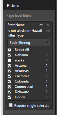
    Notice how we have data included for Alaska and Hawaii but those states are not drawn.  We want to remove the Alaska and Hawaii data points.  Add the StateName field to the Page Level Filters and then click Select All.  Now, un-check the boxes next to Alaska and Hawaii.  The data is now clean and the map correctly displays only the continental United States.

    Page Level Filters
    Page Level Filters

    Here is the filtered final map product.

    Filtered Final Map
    Filtered Final Map

    Thanks for following along.  I hope you enjoyed this tutorial.  Please share if you liked this content.  See you next week.


  • Fixing Measure Madness

    Fixing Measure Madness

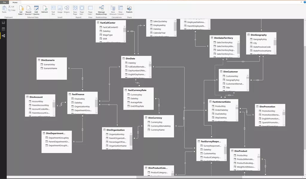
    Often times when you’re working with large data models you will have multiple tables with many relationships.  It could be complex maybe you’ve seen something like the following:

    Large Data Model
    Large Data Model – Photo Credit ( www.biinsight.com )

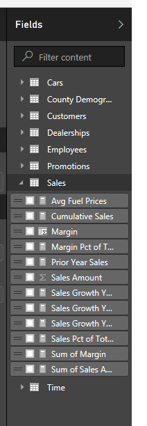
    Once all the tables have been loaded the manic measure building begins to support all the different visuals.  A couple of sums here, a number of calculates over there, and boom, a beautiful report.  You stand back and survey the work and realize you’ve built measures all over the place, in different tables, maybe even stuck a couple of measures in the wrong place.  Whoops.

    Tons of Measures
    Tons of Measures

    Maybe we should think about cleaning things up a bit, if only there was a way to group the measures.  How do I group my measures?  I’m glad you asked.  With a little trickery we can make a measure table.  Let’s begin.

    First we will load a little data.  For this tutorial we will simply copy and paste in some data.

    Note: For the full tutorial on manually entering in data visit this page.

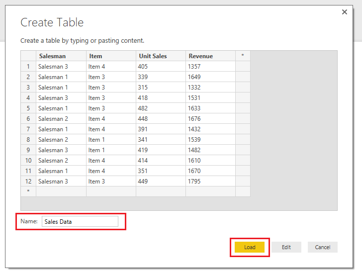
    On the Home ribbon click the Enter Data button.  Copy in the table below into the Create Table window.  Rename the table Sales Data and click Load to exit.

    Salesman Item Unit Sales Revenue
    Salesman 3 Item 4 405 1357
    Salesman 1 Item 3 339 1649
    Salesman 1 Item 3 315 1332
    Salesman 3 Item 3 418 1531
    Salesman 1 Item 3 482 1633
    Salesman 2 Item 4 448 1676
    Salesman 1 Item 4 391 1432
    Salesman 2 Item 1 341 1539
    Salesman 3 Item 1 419 1482
    Salesman 2 Item 4 414 1610
    Salesman 1 Item 4 351 1670
    Salesman 3 Item 3 449 1795
    Manually Enter Data
    Manually Enter Data

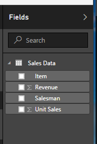
    Upon loading our data table we now have the following fields.

    Fields of Data
    Fields of Data

    Now, let’s make a measure that calculates the revenue per unit.  On the Home ribbon click the New Measure button and enter the following DAX measure.

    Revenue Per Unit = SUM('Sales Data'[Revenue]) / SUM('Sales Data'[Unit Sales])

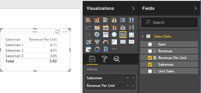
    Next, make a table with the following fields.

    Salesman Table
    Salesman Table

    Great! but, as we all know this is how the measure madness begins.  From here we refine and finesse the data to craft the data story, and end up with tons of additional tables and measures.
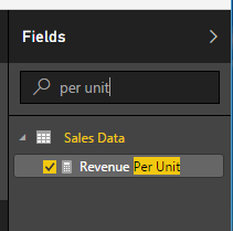
    Pro Tip: You can use the search window at the top of the Fields window to help you find buried measures or fields of data. 

    Using Search in Fields
    Using Search in Fields

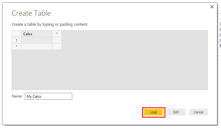
    Let’s make the measure table.  Start by clicking Enter Data on the Home ribbon.  Rename the new table to My Calcs, and rename Column1 to Calcs.   You don’t have to re-name column1, but since I’m OCD about my data I like to rename the column to the same name as the table.  Then click Load to exit the screen.

    Measure Table Load
    Measure Table Load.

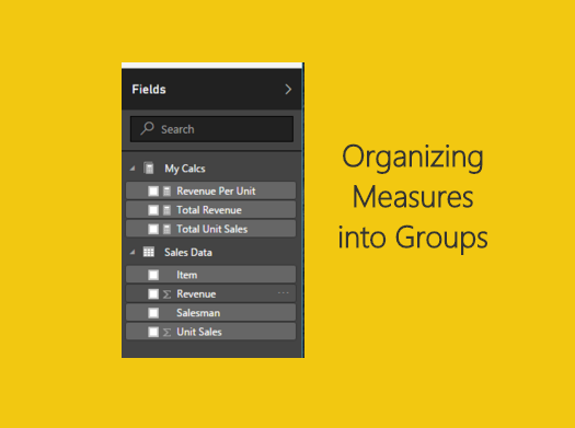
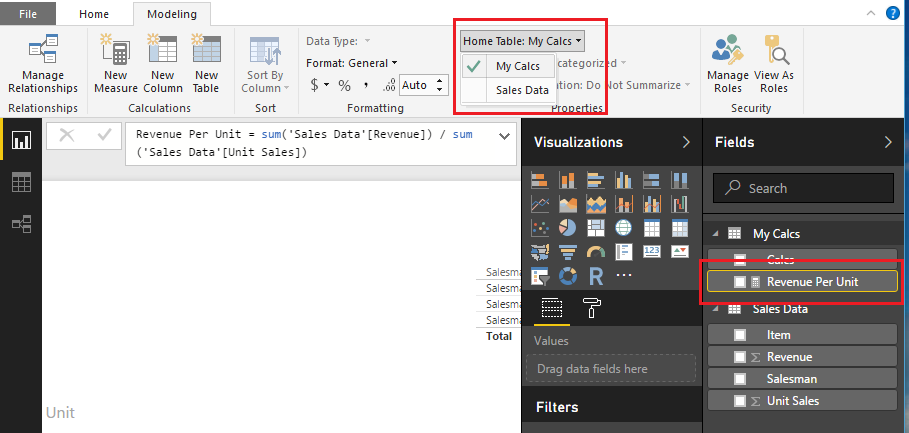
    We now have a new table labeled My Calcs with one column labeled Calcs.  Next highlight the measure we created Revenue Per Unit.  Then on the Modeling ribbon change the home table from Sales Data to My Calcs.  This will move the measure.

    Home Table for Measure
    Home Table for Measure

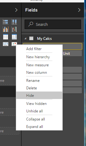
    Right click on the Calcs column in the My Calcs table and then select Hide.

    Hide Calcs Column
    Hide Calcs Column

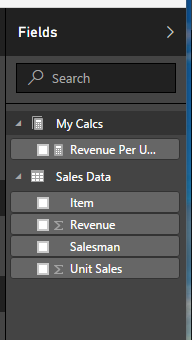
    Next Save and then reopen the document (it’s a Microsoft thing I guess).  After the document has reopened the My Calcs table has changed it’s icon from a table to a Measure icon.

    Completed Measures Table
    Completed Measures Table

    For kicks and giggles add the following measure to the My Calcs table.

    Total Revenue = SUM('Sales Data'[Revenue])

    Ok, one more.

    Total Unit Sales = SUM('Sales Data'[Unit Sales])

    There you go.  A very straight forward approach to cleaning up all the random measures in your data model.  I have found that when others team members are working with your data model this helps other people understand which fields have been calculate and which ones were imported via a query.  This also helps you group logical calculations, further creating clarity within your data model.

    If you want to read up more on making measure tables check out this great site (also linked below).  In addition to walking you through creating a measure table it also explains how to make a measure table when using direct query mode.  As the article explains, while you are in direct query mode you are unable to manually enter data.  Nice job, Soheil Bakhshi, well done.

    How to Define A Measure Table in Power BI Desktop

    If you want to take your DAX skills to the next level, try jumping into this book by Rob Collie and Avichal Singh.  It’s an easy read but very insightful.

    If you liked this tutorial make sure you share.  See you next week!
     

  • Intro to Guy In a Cube

    Intro to Guy In a Cube

    Kicking off my video series for PowerBI.Tips I have to give incredible props to Adam Saxton.  Adam is a Microsoft Employee who creates THE BEST content for PowerBI.  There are a lot of videos out on the internet that are interesting and helpful to learn from.  However, Adam takes it to another level.  The videos are relatively short and packed with useful information.  Below is the introduction video to Adam who is The Guy in a Cube.

    I will be definitely sharing more videos from Adam in the future!

  • Using Advanced Mapping in ArcGIS Preview

    Using Advanced Mapping in ArcGIS Preview

    In the September 2016 release of PowerBI, Microsoft introduced a new visual called the ArcGIS Maps preview.  For more information on the maps integration you can read the following post from Microsoft.  This tutorial will review how to load data using Latitude and Longitude data and map those points on the ArcGIS map.

    First, we need to open PowerBI Desktop and then we will load some data.  The version of PowerBI Desktop for this tutorial is 2.39.4526.362 64-bit (September, 2016).  You can download the latest version of the software here.

    On the Home ribbon click on the Get Data button and from the Get Data window select Blank Query.  Click Connect to proceed.

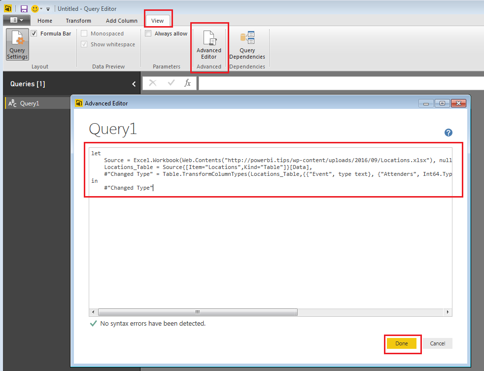
    Now you will be in the Query Editor, click on the View ribbon and select the Advanced Editor button.  The Advanced Editor will now open.

    Enter the following code into the Advanced Editor: (you can copy and paste the code directly from this site)  Click Done to load the data.

    let
     Source = Excel.Workbook(Web.Contents("https://powerbitips03.blob.core.windows.net/blobpowerbitips03/wp-content/uploads/2016/09/Locations.xlsx"), null, true),
     Locations_Table = Source{[Item="Locations",Kind="Table"]}[Data],
     #"Changed Type" = Table.TransformColumnTypes(Locations_Table,{{"Event", type text}, {"Attenders", Int64.Type}, {"Zip", Int64.Type}, {"Latitude", type number}, {"Longitude", type number}})
    in
     #"Changed Type"

    Note: this will load an excel file that is hosted on PowerBI.Tips, so make sure you have an internet connection.

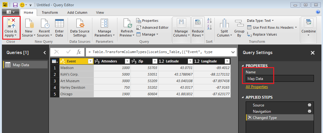
    Load Map Data
    Load Query

    Re-name your query to Map Data and then on the Home ribbon click Close & Apply.

    Load Map Data In PBI
    Load Map Data In PBI

    Before working on this tutorial, you will want to make sure you have enabled the ArcGIS map which is in preview.

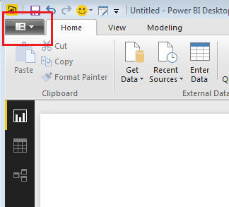
    Click the Menu button to open up the menu options.

    PBI Menu Button
    PBI Menu Button

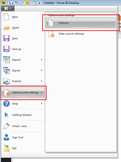
    This will expose the menu.  With the menu open click on Options and Settings and then click on Options.

    Selecting Options
    Selecting Options

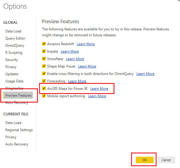
    Once the Options menu is open, click on Preview Features and then make sure the ArcGIS Maps for PowerBI preview feature is check.  Then click OK to close the options menu.

    Options Menu
    Options Menu

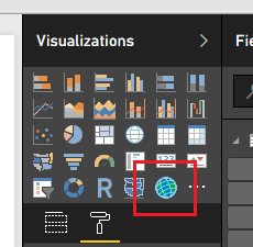
    You should now see a new bright blue icon listed in the Visualizations window.

    ArcGIS Maps Icon
    ArcGIS Maps Icon

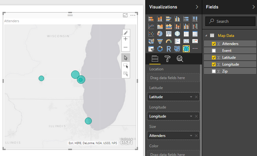
    Click on the ArcGIS visualization and then add the following following columns of data from the Fields window into the visual.

    Fields for ArcGIS Map
    Fields for ArcGIS Map

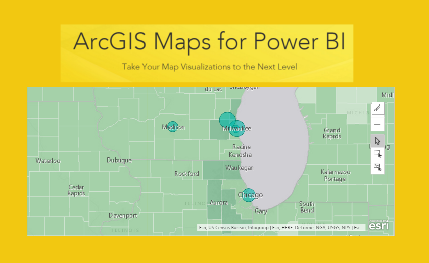
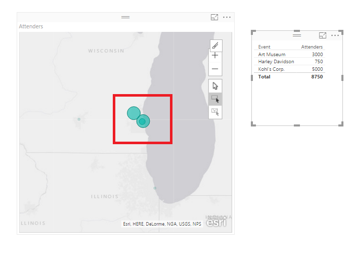
    OK, Wow, seems like a normal map.  So, why all the hype?  Well, unlike other mapping visualizations, this map enhances the selection methods for points on a map.

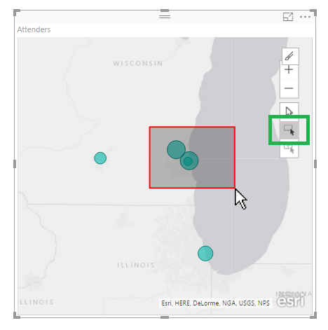
    By clicking on the square with the black mouse arrow (highlighted with a green box here because the selection tool for the visual uses a red box)  You can then click drag a red box across the map to select multiple geographical points on the map.

    Highlighting Points on Map
    Highlighting Points on Map

    Selecting points on the map will filter other visuals on the page.

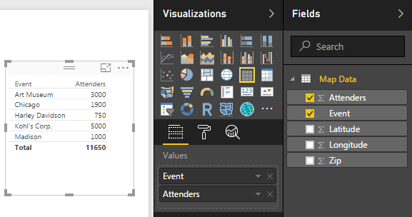
    Add a Table visual with the following fields:

    Table Visual Fields
    Table Visual Fields

    Now click the Multi-Select button and highlight some points on the map.

    Multi-Select Button
    Multi-Select Button

    Notice how only the selected points are highlighted on the map and the table filters to only those points.

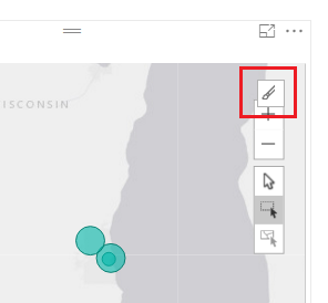
    To enhance the map further click the In-Focus Edit Mode button.

    In-Focus Edit Mode
    In-Focus Edit Mode

    Now, the map editor opens.  This allows you to change the basemap view, the theme of the map, symbols on the map and adds other data to enhance the coloring of the map.

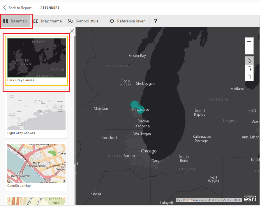
    Click on the Basemap button and then select the Dark Gray Canvas.  We have turned the map in to a sort of night mode.

    Basemap Change
    Basemap Change

    Have fun here and explore a couple of the other map types.

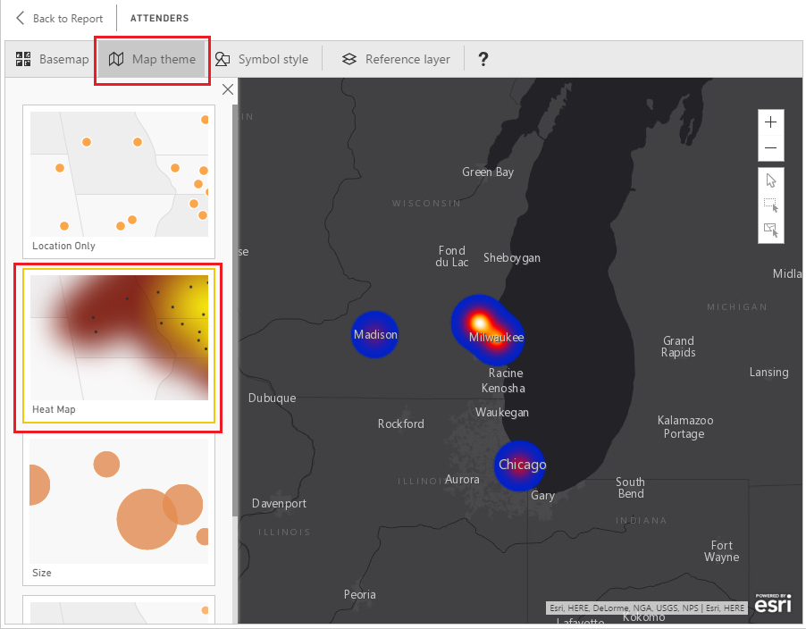
    Next Click on the Map Theme then click on the Heat Map.  Alright, this is getting pretty cool.

    Heat Map Selection
    Heat Map Selection

    In the next section Symbol Style you can change the properties of the points on the map.  For the heat map you can change the Transparency and the Area of Influence of the points.  Each map theme, Location, Heat Map, Size, and Clustering have different Symbol Style properties.  So you might want to select a couple different Map Themes and try adjusting the Symbol Styles to see how they change.

    Now finally, the best part of the ArcGIS mapping, the Reference Layer.  This will blow your mind!

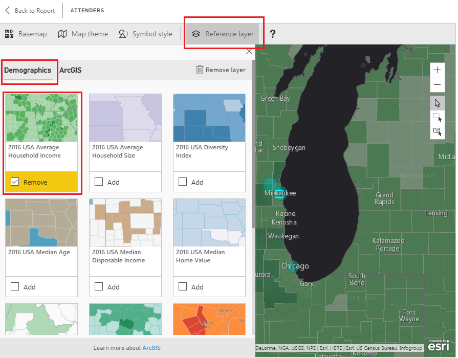
    Click the Reference layer button then select a layer to add from the Demographics tab.  For this example, I chose the USA Average Household Income.

    Household Income Layer
    Household Income Layer

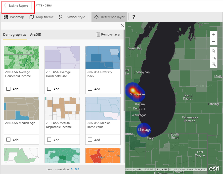
    To return to the Report click the Back to Report button in the upper left hand corner of the page view.

    Back to Report
    Back to Report

    The layer feature is by far the most helpful part of this tool.  Imagine the time required to collect all that regional demographics data, model it and then to apply it to the mapping visual.  The ArcGIS mapping tool is quite impressive.

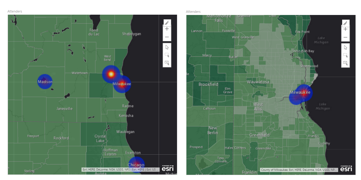
    One other note before we leave.  Now that you are back on the report level view.  Use your mouse scrolling wheel and zoom in and out on the map visual.  Notice the closer you zoom into the data points the more detailed the regional views become. See comparison below:

    Zoomed Views
    Zoomed Views

    Thanks for following along.  Remember to share if you liked this tutorial.  See you next week.

  • HexBin Plot using R

    HexBin Plot using R

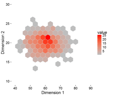
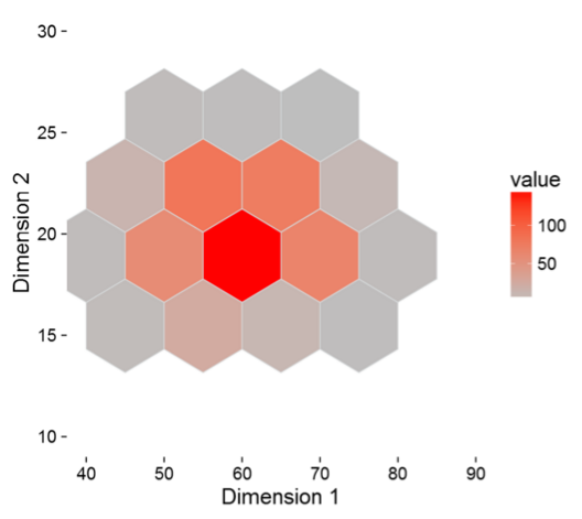
    Continuing on the theme with R this month, this week tutorial will be to design a hexagonal bin plot.  At first you may say what in the world is a hexagonal bin plot.  I’m glad you asked, behold a sweet honey comb of data:

    Hexbin Plot
    Hexagonal Bin Plot

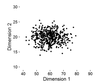
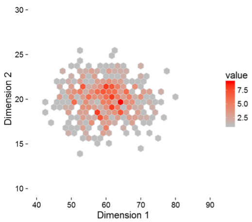
    The hexagonal bin plot looks just like a honey comb with different shading.   In this plot we have a number of data points with are graphed in two dimensions (Dimension 1, x-axis and Dimension 2, y-axis).  Each hexagon square represents a collection of points.  Now, if we plot only the points on the same graph we have the following.

    Scatter Plot
    Scatter Plot

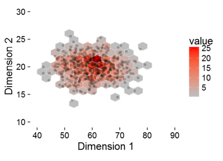
    In the scatter plot, it’s difficult to see the concentration of points and if there is any correlation between the first dimension and the second dimension.  By comparison, the hex bin plot counts all the points and plots a heat map.  And, if you ask me the hexagonal bin plot just looks better visually.  To bring this all together, if we overlay the scatter plot on top of the hexagonal bin plot you can see that the higher concentration of dots are in the shaded areas with darker red.

    Plot Overlay
    Plot Overlay

    Cool, now lets build some visuals.  Lets begin.  Tutorial <- Hexagonal Bin Plot   (sorry had to interject a bit of R humor here, ignore if you don’t like code humor)

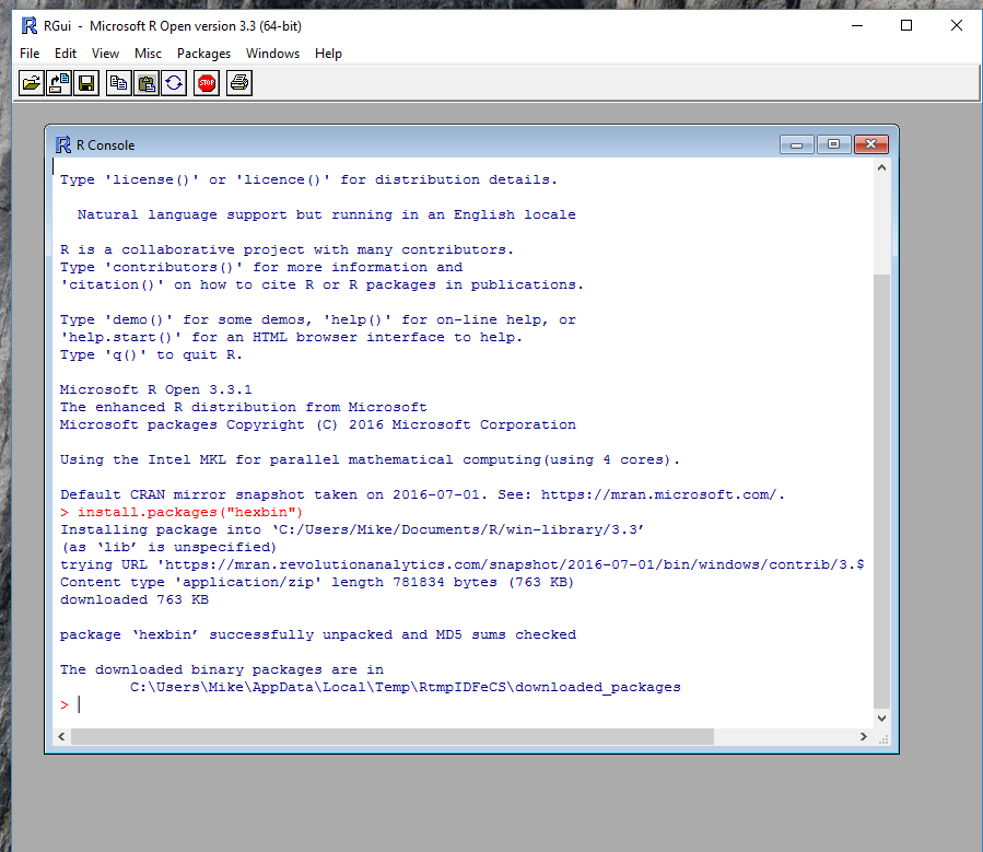
    The very first step will be to open the R console and to install a new library called HexBin.  Run the following code in the Mircosoft RGui.

    install.packages("hexbin")

    This will load the correct library for use within PowerBI.

    Install hexbin
    Install hexbin

    Start by opening up PowerBI.  Click on the Get Data button on the home ribbon, then select Blank Query.  In the Query editor click on the View ribbon and click on the Advanced Editor.  Enter the following query into the Advanced Editor:

    let
     Source = Csv.Document(Web.Contents("https://powerbitips03.blob.core.windows.net/blobpowerbitips03/wp-content/uploads/2016/09/Hexabin-Data.csv"),[Delimiter=",", Columns=3, Encoding=1252, QuoteStyle=QuoteStyle.None]),
     #"Promoted Headers" = Table.PromoteHeaders(Source),
     #"Changed Type" = Table.TransformColumnTypes(#"Promoted Headers",{{"SampleID", Int64.Type}, {"Xvalues", type number}, {"Yvalues", type number}})
    in
     #"Changed Type"

    This query loads a csv file of data into PowerBI.

    Note:  For more information on how to open and copy and paste M language into the Advanced Editor you can follow this tutorial, which will walk you though the steps.

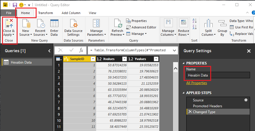
    After the clicking Done in the Advanced Editor the data will load.  Next rename the query to Hexabin Data and then on the Home ribbon click Close & Apply.

    Save Query
    Save Query

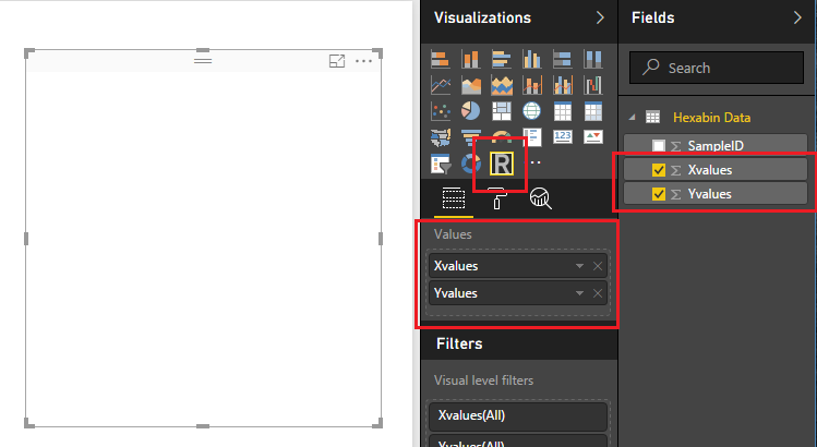
    Next click on the R visual in the Visualizations bar on the right side of the screen.  There will likely be a pop up warning you about enabling R Scripts.  Click Enable to activate the R script editor.  With the R script visual selected on the page add the following columns to the Values field selector.

    R Visual Fields
    R Visual Fields

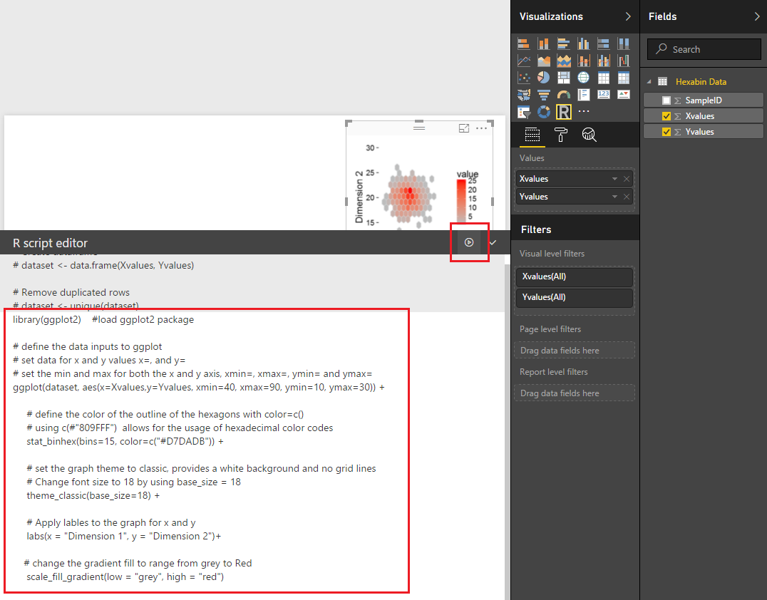
    Notice that the R visual is blank at this time.  Next add the following R code in the R script editor window.  This will tell PowerBI Desktop to load the ggplot2 library and define all the parameters for the plot.  I’ve added comments to the code using # symbols.

    library(ggplot2) #load ggplot2 package
    
    # define the data inputs to ggplot
     # set data for x and y values x=, and y=
     # set the min and max for both the x and y axis, xmin=, xmax=, ymin= and ymax=
     ggplot(dataset, aes(x=Xvalues,y=Yvalues, xmin=40, xmax=90, ymin=10, ymax=30)) +
    
    # define the color of the outline of the hexagons with color=c()
     # using c(#"809FFF") allows for the usage of hexadecimal color codes
     stat_binhex(bins=15, color=c("#D7DADB")) +
    
    # set the graph theme to classic, provides a white background and no grid lines
     # Change font size to 18 by using base_size = 18
     theme_classic(base_size=18) +
    
    # Apply lables to the graph for x and y
     labs(x = "Dimension 1", y = "Dimension 2")+
    
    # change the gradient fill to range from grey to Red
     scale_fill_gradient(low = "grey", high = "red")

    Click the run button and the code will execute revealing our new plot.

    R Script Code
    R Script Code

    One area of the code that is interesting to change is the section talking about the number of bins.  In the code pasted above the code states there are 15 bins.

    stat_binhex(bins=15, color=c("#D7DADB")) +

    Try increasing this number and decreasing this number to see what happens with the plot.

    Five Bins
    Five Bins
    stat_binhex(bins=5, color=c("#D7DADB")) +
    Thirty Bins
    Thirty Bins
    stat_binhex(bins=30, color=c("#D7DADB")) +

    Well that is it.  Thanks for reading through another tutorial.  I hope you had fun.

    Want to see more R checkout the Microsoft R Script Showcase.  If you want to download the PBIX file used to create this visual you can download the file here.

    If you want to learn more about R and the different visuals you can build within R check out this great book which helped me learn plotting with R.

  • Digging Deeper with R Visuals for PowerBI

    Digging Deeper with R Visuals for PowerBI

    Back by popular demand, we have another great tutorial on using R visuals.  There are a number of amazing visuals that have been supplied with the PowerBI desktop tool.  However, there are some limitations.  For example you can’t merge a scatter plot with a bar chart or with a area chart.  In some cases it may be applicable to display one graph with multiple plot types.  Now, to be fair Power BI desktop does supply you with a bar chart and line chart, Kudos Microsoft, #Winning…. but, I want more.

    This brings me to the need to learn R Visuals in PowerBI.  I’ve been interested in learning R and working on understanding how to leverage the drawing capabilities of R inside PowerBI.  Microsoft recently deployed the R Script Showcase, which has excellent examples of R scripts.  I took it upon myself to start learning.  Here is what I came up with.

    R Plot in PowerBI Desktop
    R Plot in PowerBI Desktop

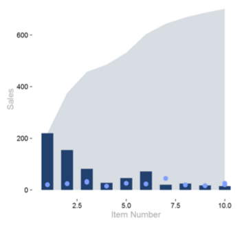
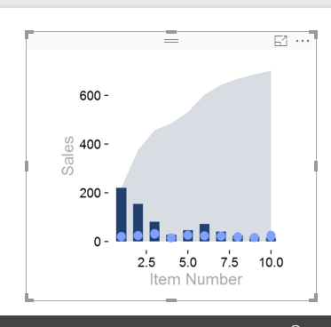
    This is an area plot in the background, a bar chart as a middle layer and dots for each bar.  The use case for this type of plot would be to plot sales by item number,  sales are in the dark blue bars, and the price is shown as the light blue dots.  The area behind the bars represent a running total of all sales for all items.  Thus, when you reach item number 10, the area represents 100% of all sales for all items listed.

    If you want to download my R visual script included in the sample pbix file you can do so here.

    Great, lets start the tutorial.

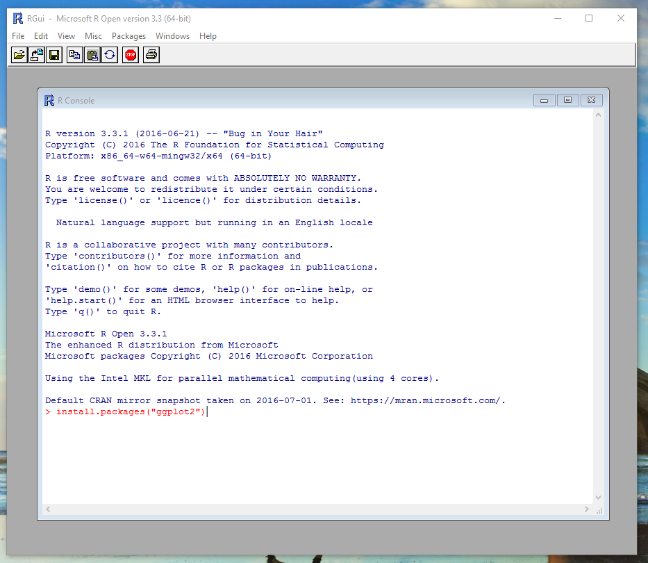
    First you will need to make sure you have installed R on your computer.  To see how to do this you can follow my earlier post about installing R from Microsoft Open R project.  Once you’ve installed R open up the R console and enter the following code to install the ggplot2 package.

    install.packages("ggplot2")
    Install ggplot2 Code
    Install ggplot2 Code

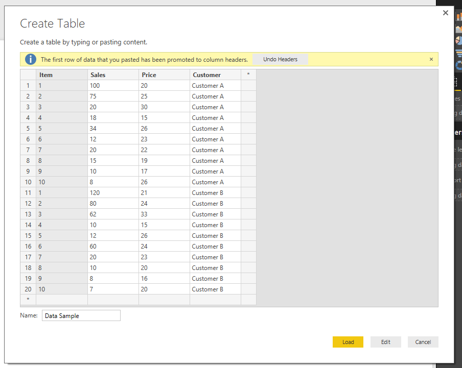
    Once complete you can close the R console and enter PowerBI Desktop.  First, we will acquire some data to work with.  Click on the Home ribbon and then  select Enter Data.  You will be presented with the Create Table dialog box.  Copy and paste the following table of information into the dialog box.

    Item Sales Price Customer
    1 100 20 Customer A
    2 75 25 Customer A
    3 20 30 Customer A
    4 18 15 Customer A
    5 34 26 Customer A
    6 12 23 Customer A
    7 20 22 Customer A
    8 15 19 Customer A
    9 10 17 Customer A
    10 8 26 Customer A
    1 120 21 Customer B
    2 80 24 Customer B
    3 62 33 Customer B
    4 10 15 Customer B
    5 12 26 Customer B
    6 60 24 Customer B
    7 20 23 Customer B
    8 10 20 Customer B
    9 8 16 Customer B
    10 7 20 Customer B

    Rename your table to be titled Data Sample.

    datatable
    Data Sample Table

    Click Load to bring in the data into PowerBI.

    Next, we will need to create a cumulative calculated column measure using DAX.  On the home ribbon click the New Measure button and enter the following DAX expression.

    Cumulative = CALCULATE(  sum('Data Sample'[Sales] ) ,   FILTERS(  'Data Sample'[Customer] ) ,  FILTER( all( 'Data Sample' )  ,  'Data Sample'[Item] <= MAX( 'Data Sample'[Item] ) ) )

    This creates column value that adds all the sales of the items below the selected row.  For example if I’m calculating the cumulative total for item three, the sum() will add every item that is three and lower.

    Now, add the R visual by clicking on the R icon in the Visualizations window.

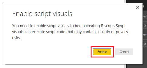
    Note: There will be an approval window that will require you to enable the R script visuals.  Click Enable to proceed.

    Enable R Visuals
    Enable R Visuals

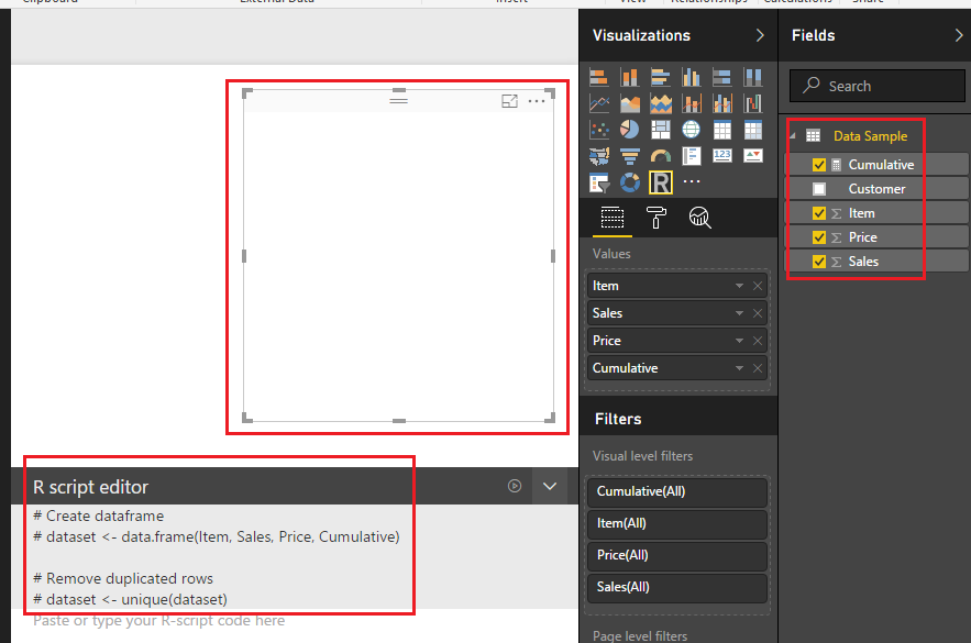
    While selecting the R visual add the following columns to the Values field in the Visualization window.

    Add Column Data
    Add Column Data

    Note: After you add the columns to the Values the R visual renders a blank image.  Additionally, there is automatic comments entered into the R Script Editor (the # sign is a designation that denotes a text phrase).

    Next, enter the following R code into the script editor.

    library(ggplot2)   # include this package to use Graphing functions below
    
    ggplot(dataset, aes(xmin=1, x=Item)) +    # Initialize ggplot function, define the x axis with Item data
     geom_ribbon(fill=c("#D7DDE2"),           # Set the color of the Area Plot,
     aes( ymin=0, ymax=Cumulative )) +        # Define the Y-Axis data
     geom_bar(fill=c("#21406D") ,             # Define the color of the Bars
     stat = "identity" ,      # Define the Statatics property of the bars - This is a required field
     width=.6 ,               # Change the bar width to 60% - 1 would be full bar width
     aes( x=Item, y=Sales )) +          # Define the X and Y axis for bars
     geom_point( color=c("#809FFF"),    # Define the color of the dots
     size=4,                  # Define the dot size
     aes( x=Item, y=Price )) +          # Define the X and Y axis values
     theme_classic(base_size=18) +      # Remove unwanted items from plot area such as grid lines and X and Y axis lines, Change font size to 18
     theme( axis.title.x = element_text(colour = "dark grey"),     # Define the X axis text color
     axis.title.y = element_text(colour = "dark grey")) +          # Define the Y axis text color
     labs( x="Item Number", y="Sales")                             # Define the labels of the X and Y Axis

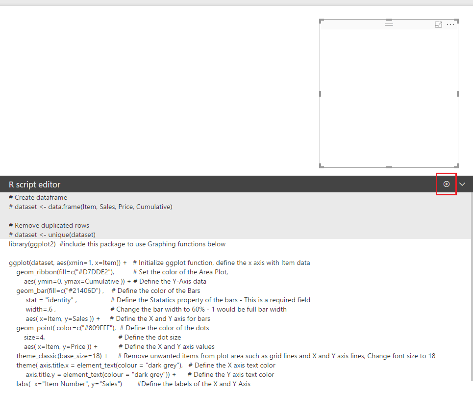
    Press the execute R Script button which is located on the right side of the R Script Editor bar.

    Execute R Script Editor Button
    Execute R Script Editor Button

    The R Script will execute and the plot will be generated.

    R Plot Generation
    R Plot Generation


    Great, we have completed a R visual.  So what, why is this such a big deal.  Well, it is because the R Script will execute every time a filter is applied or changed.  Lets see it in action.

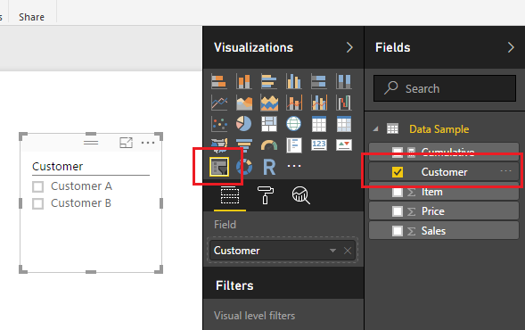
    Add a slicer with the Customer column.

    Add Customer Slicer
    Add Customer Slicer

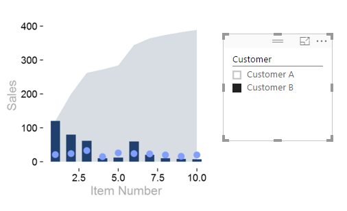
    Notice when you select the different customers, either A or B the R script Visual will change to reflect the selected customer.

    Customer B Selected
    Customer B Selected

    Now you can write the R script code once and use the filtering that is native in PowerBI to quickly change the data frame supporting the R Visuals.

    As always, thanks for following along.  Don’t forget to share if you liked this tutorial.

    Want to learn more about PowerBI and Using DAX.  Check out this great book from Rob Collie talking the power of DAX.  The book covers topics applicable for both PowerBI and Power Pivot inside excel.  I’ve personally read it and Rob has a great way of interjecting some fun humor while teaching you the essentials of DAX.