Measures – Dynamic CAGR Calculation in DAX

CAGR
CAGR

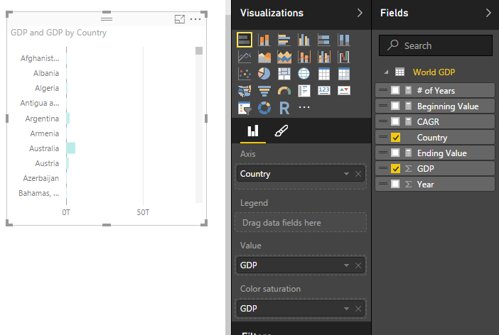
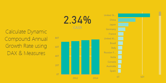
This tutorial walks through calculating a dynamic Compound Annual Growth Rate (CAGR).  By dynamic we mean as you select different items on a bar chart for example the CAGR calculation will update to reveal the CAGR calculation only for the selected data.  See the example below:

Lets start off by getting some data.  For this tutorial we will gather data from World Bank found here.  To make this process less about acquiring data and more about calculating the CAGR. Below is the Query Editor code you can copy and paste directly into the Advance Editor.

let
 Source = Excel.Workbook(Web.Contents("https://powerbi.tips/wp-content/uploads/2017/11/Worldbank-DataSet.xlsx"), null, true),
 EconomicData_Table = Source{[Item="EconomicData",Kind="Table"]}[Data],
 #"Changed Type" = Table.TransformColumnTypes(EconomicData_Table,{{"Country Name", type text}, {"Country Code", type text}, {"Indicator Name", type text}, {"Indicator Code", type text}, {"1960", type number}, {"1961", type number}, {"1962", type number}, {"1963", type number}, {"1964", type number}, {"1965", type number}, {"1966", type number}, {"1967", type number}, {"1968", type number}, {"1969", type number}, {"1970", type number}, {"1971", type number}, {"1972", type number}, {"1973", type number}, {"1974", type number}, {"1975", type number}, {"1976", type number}, {"1977", type number}, {"1978", type number}, {"1979", type number}, {"1980", type number}, {"1981", type number}, {"1982", type number}, {"1983", type number}, {"1984", type number}, {"1985", type number}, {"1986", type number}, {"1987", type number}, {"1988", type number}, {"1989", type number}, {"1990", type number}, {"1991", type number}, {"1992", type number}, {"1993", type number}, {"1994", type number}, {"1995", type number}, {"1996", type number}, {"1997", type number}, {"1998", type number}, {"1999", type number}, {"2000", type number}, {"2001", type number}, {"2002", type number}, {"2003", type number}, {"2004", type number}, {"2005", type number}, {"2006", type number}, {"2007", type number}, {"2008", type number}, {"2009", type number}, {"2010", type number}, {"2011", type number}, {"2012", type number}, {"2013", type number}, {"2014", type number}, {"2015", type number}, {"2016", type number}, {"2017", type any}}),
 #"Removed Other Columns" = Table.SelectColumns(#"Changed Type",{"Country Name", "2011", "2012", "2013", "2014", "2015", "2016"}),
 #"Filtered Rows" = Table.SelectRows(#"Removed Other Columns", each [2011] <> null and [2012] <> null and [2013] <> null and [2014] <> null and [2015] <> null and [2016] <> null),
 #"Unpivoted Other Columns" = Table.UnpivotOtherColumns(#"Filtered Rows", {"Country Name"}, "Attribute", "Value"),
 #"Renamed Columns" = Table.RenameColumns(#"Unpivoted Other Columns",{{"Country Name", "Country"}, {"Attribute", "Year"}, {"Value", "GDP"}})
in
 #"Renamed Columns"

Note: The tutorial on how to copy and paste the code into the Query Editor is located here.

Paste the code above into the advance editor.  Click Done to load the query into the the Query Editor.  Rename the Query to World GDP and then on the home ribbon click Close & Apply.
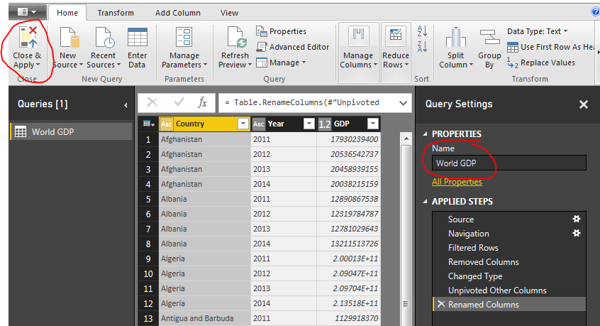
World GDP Query
World GDP Query

Loading the query loads the following columns into the fields bar on the right hand side of the screen.
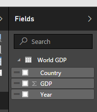
Fields Load from World GDP

Next we will build a number of measure that will calculate the required variables to be used in our CAGR calculation.  For reference the CAGR calculation is as follows: (found from investopia.com)

CAGR Calculation Image
CAGR Calculation

For each variable on the right of the equation we will create one measure ; one for Ending Value, Beginning Value and # of Years.  On the Home ribbon click the button labeled New Measure.  Enter the following equation for the beginning value:

Beginning Value = CALCULATE(SUM('World GDP'[GDP]),FILTER('World GDP','World GDP'[Year]=MIN('World GDP'[Year])))

This equation totals all the items in the table called World GDP in the column labeled GDP.  This calculation will change based on the selections in the page view.

Add two more measures for Ending Value and # of years

Ending Value = CALCULATE(SUM('World GDP'[GDP]),FILTER('World GDP','World GDP'[Year]=MAX('World GDP'[Year])))
# of Years = (MAX('World GDP'[Year])-MIN('World GDP'[Year]))

Your fields list should now look like the following:
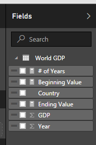
Fields List with Measures

Next add a Card visual for each new measure we added.  A measure is illustrated by the little calculator image next to the measure.  I have highlighted the Ending Value measure as a card for an example.
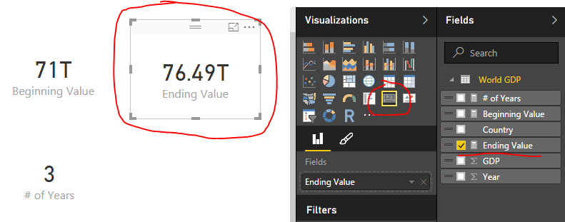
Ending Value Measure as Card Visual

Combining all the previous measures we will now calculate the CAGR value.  Add one final measure and add the following equation to calculate CAGR:

CAGR = ([Ending Value]/[Beginning Value])^(1/[# of Years])-1

This calculation uses the prior three measures we created.  Add the CAGR as a card visual to the page.
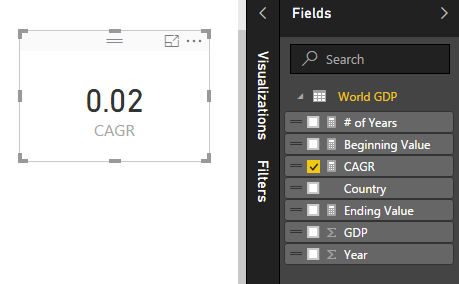
Card Visual for CAGR

Notice how the value of this measure is listed as a decimal, which isn’t very useful.  To change this to a percentage click on the measure CAGR item in the Fields list. Then on the Modeling ribbon change the format from General to Percentage.
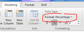
Format Change to Percentage

This changes the card visual to now be in a percentage format.
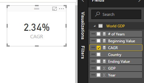
Percentage Format
Percentage Format

Now you can add some fun visuals to the page and depending on what is selected the CAGR will change depending on the selected values.

ProTip: To calculate the CAGR you can alternatively compute the entire calculation into one large measure like so:

CAGR = ( [Ending Value] / [Beginning Value] )^(1/ [# of Years] )-1

is the same as below:

CAGR = (  CALCULATE(SUM('World GDP'[GDP]),FILTER('World GDP','World GDP'[Year]=MAX('World GDP'[Year])))  /  CALCULATE(SUM('World GDP'[GDP]),FILTER('World GDP','World GDP'[Year]=MIN('World GDP'[Year]))) ) ^ (1/  (MAX('World GDP'[Year])-MIN('World GDP'[Year]))  )-1

A final recommendation is to wrap the CAGR calculation in an IFERROR function to make sure if one year is selected the measure doesn’t fail.  This returns a 0 if there is a calculation error of the equation. Documentation on IFERROR is found here.

CAGR = IFERROR( ([Ending Value]/[Beginning Value])^(1/[# of Years])-1 , 0)

To finish out the tutorial you can add the following visuals:
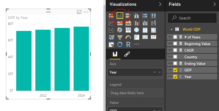
Stacked Bar Chart Visual
Stacked Bar Chart Visual – GDP by Year
GDP by Country
Stacked Bar Chart Visual – GDP by Country

Note: you can sort the items in the stacked bar chart by selecting the ellipsis (the three dots in the upper right hand corner) and then selecting Sort By and clicking GDP.
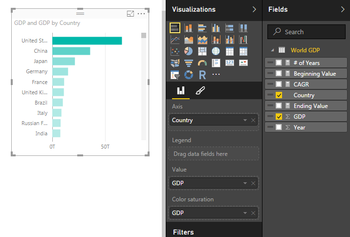
Country Sorted by GDP

Finally select different items in the GDP by Year chart or the GDP by Country chart.  To select more than one item in the bar charts you have hold shift and left mouse click the multiple items.  Notice how all the measures change.
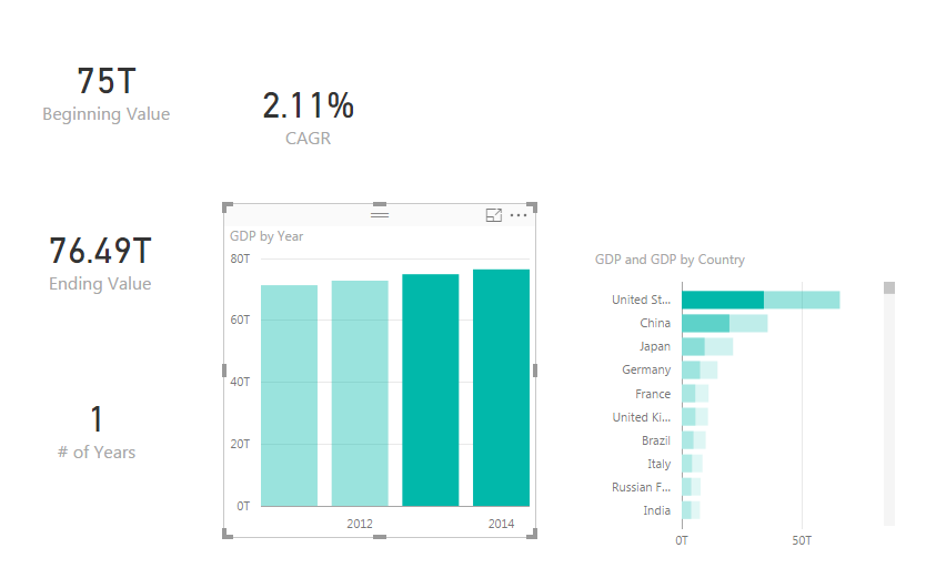
Years 2013 & 2014 CAGR

Thanks for following along.

This tutorial used the following materials:

Want to learn more about PowerBI and Using DAX.  Check out this great book from Rob Collie talking the power of DAX.  The book covers topics applicable for both PowerBI and Power Pivot inside excel.  I’ve personally read it and Rob has a great way of interjecting some fun humor while teaching you the essentials of DAX.

9 Comments

  1. I would like a line graph that shows the percentage change of the COUNT of employee ID’s in a column over a span of 16 quarters. I’m wondering if you could provide some assistance?

    • Ok, I have done some research on what you were asking. Maybe this will help.

      There is an assumption here that you have a list of employee IDs and Dates similar to the following table:
      Date | Employee ID
      1/1/2016 123
      1/1/2016 456
      1/2/2016 123
      1/2/2016 456
      1/3/2016 123
      1/4/2016 123
      1/4/2016 789

      Thus, the count for Badge 123 would be in total 4, it appeared every in every date.
      For badge 456 the count would be 2.

      This can be simply done with a measure something like:
      Count of Badges = Count( EmployeeID )
      Then in your visual you’d use the Employee ID and your new measure Count of Badges in a table
      This would yield:
      Employee ID | Count of Badges
      123 4
      456 2
      789 1

      When you mention % change it gets much more difficult. Now you have to determine how the percent change will operate.
      For our example you have a date range of 4 days. 1/1 to 1/4 for percent change you want to calculate the total of the first 2 days then compare compare to the second two. This is when the measure come in handy. To do this I calculate everything off the Max date.
      The measure would look like the following:
      Max Date = Max( Date )

      Then Calculate the Min date:
      Min Date = Min( Date)

      Count the number of days between dates:
      Date Delta = [Min Date] – [Max Date]

      Calculate half of the time range:
      Half Time Range = RoundDown( [Date Delta]/2 , 0 )
      – you do this because there will be time periods when there are an odd number of days, for example if your time period was 35 you would have to calculate your percent change between 17.5 days, this doesn’t make sense. Thus you round down, so when the time period is an odd number half the time period is a whole number. This makes 35 rounded down to 17 days.

      Calculate the middle date of the % change time period:
      Middle Date = [Max Date] – [Half Time Range]

      Calculate the end date:
      End Date = [Middle Date] – [Half Time Range]

      now we calculate the count of IDs with the date ranges we determined,
      Note: Period 1 Date range should be counting the values between [Max Date] and [Middle Date] and Period 2 Date range should be counting the values between [Middle Date] and [End Date]

      Create new measures
      Period 1 = Calculate( Count( Date ) , DatesBetween( Table , [Middle] , [Max Date] ) )
      Period 2 = Calculate( Count( Date ) , DatesBetween( Table , [End Date] , [Middle Date] )

      finally calculate your % change
      % change = Divide( [Period 1], [Period 2]) – 1

      Hope that helps.
      Mike

  2. Dear Mike
    I am new to this blog. my apologies, if I am too direct.
    I have a problem for which I am unable to find a solution. I was wondering if you could give some solution, would be really appreciative.
    I am working in excel powerpivot, have slight knowledge of DAX.
    I have a table in which I have userIDs, and their level play details. The details include level no, start time and end time of each level. I want to calculate the session count and approx duration for each session.
    The sessions will be ofcourse for each individual user ID.
    A Session will/can include multiple levels, I am taking all levels that start within 5 minutes of completion of previous level as one sesssion.

    Waiting for any and all guidance.

    Best Regards/Aamer

    • This is a really tricky one. I think within PowerBI or Excel you could calculate the duration of each level. However, when you want to string together a number of user sessions and designate a time window of 5 minutes between each session your working with an indefinite amount. For example user 123 could have played level 1 (4min), 2 (3min), and 3 (5 min), for a total time of 15 minutes. From what i read above this would be a session. However, because of the way your data is structured you have to compare every end time to start time where the user id is the same. This now becomes more of a question that would have to be solved inside a database. I am not a aware of any methods that exist today that would let you build a session for a user.

      If I were going to build I would have to run the data through some sort of SQL data warehouse to aggregate the session info.

      Sorry that probably wasn’t to helpful. Good luck on your game.

  3. Hi Mike,
    I am trying to rework your data and steps but I get an error which I cannot resolve myself…
    the error is just after having copied and pasted the query text into the advanced editor. The action starts and stop at Removed columns:

    = Table.RemoveColumns(#”Filtered Rows”,{“”, “2”})

    and in yellow:
    Expression.Error: The column ” of the table wasn’t found.
    Details:

    when I remove the step to remove columns another error occurs: 2011 is missing…

    so I started looking at the data source and apparently the url you used now contains very little data:

    Kind Name Text
    Element HTML *blank*

    Is there some way of getting insight into the correct webaddress – I do understand you depend on that source, but how to get to the right table would probably solve this item…

    Thanks for your tutorials so far and kind regards, Henrike

    • HI Henrike,

      You can use below link for Web “http://databank.worldbank.org/data/reports.aspx?source=2&series=NY.GDP.MKTP.PP.KD&country=”

  4. Hi Mike,
    I am unable to get the data for the exercise but did manage to download the .csv file and after some removing of columns, transposing and fill-ing of data I have a file with a row for each country and a column for each year. Is there a way in PowerBI to get this in the Year, Country GDP format you use for the exercise?

    • I’m so sorry, the website has since changed how it stores it’s data. Thus, my old query no longer works. I have updated the query in the blog post. Also, Here is a copy of the new Query that you can enter into M:
      let
      Source = Excel.Workbook(Web.Contents(“https://powerbi.tips/wp-content/uploads/2017/11/Worldbank-DataSet.xlsx”), null, true),
      EconomicData_Table = Source{[Item=”EconomicData”,Kind=”Table”]}[Data],
      #”Changed Type” = Table.TransformColumnTypes(EconomicData_Table,{{“Country Name”, type text}, {“Country Code”, type text}, {“Indicator Name”, type text}, {“Indicator Code”, type text}, {“1960”, type number}, {“1961”, type number}, {“1962”, type number}, {“1963”, type number}, {“1964”, type number}, {“1965”, type number}, {“1966”, type number}, {“1967”, type number}, {“1968”, type number}, {“1969”, type number}, {“1970”, type number}, {“1971”, type number}, {“1972”, type number}, {“1973”, type number}, {“1974”, type number}, {“1975”, type number}, {“1976”, type number}, {“1977”, type number}, {“1978”, type number}, {“1979”, type number}, {“1980”, type number}, {“1981”, type number}, {“1982”, type number}, {“1983”, type number}, {“1984”, type number}, {“1985”, type number}, {“1986”, type number}, {“1987”, type number}, {“1988”, type number}, {“1989”, type number}, {“1990”, type number}, {“1991”, type number}, {“1992”, type number}, {“1993”, type number}, {“1994”, type number}, {“1995”, type number}, {“1996”, type number}, {“1997”, type number}, {“1998”, type number}, {“1999”, type number}, {“2000”, type number}, {“2001”, type number}, {“2002”, type number}, {“2003”, type number}, {“2004”, type number}, {“2005”, type number}, {“2006”, type number}, {“2007”, type number}, {“2008”, type number}, {“2009”, type number}, {“2010”, type number}, {“2011”, type number}, {“2012”, type number}, {“2013”, type number}, {“2014”, type number}, {“2015”, type number}, {“2016”, type number}, {“2017″, type any}}),
      #”Removed Other Columns” = Table.SelectColumns(#”Changed Type”,{“Country Name”, “2011”, “2012”, “2013”, “2014”, “2015”, “2016”}),
      #”Filtered Rows” = Table.SelectRows(#”Removed Other Columns”, each [2011] <> null and [2012] <> null and [2013] <> null and [2014] <> null and [2015] <> null and [2016] <> null),
      #”Unpivoted Other Columns” = Table.UnpivotOtherColumns(#”Filtered Rows”, {“Country Name”}, “Attribute”, “Value”),
      #”Renamed Columns” = Table.RenameColumns(#”Unpivoted Other Columns”,{{“Country Name”, “Country”}, {“Attribute”, “Year”}, {“Value”, “GDP”}})
      in
      #”Renamed Columns”

      This should allow you to complete the tutorial.

1 Trackback / Pingback

  1. #Excel Super Links #43 – shared by David Hager | Excel For You

Comments are closed.