
I had an interesting comment come up in conversation about how to calculate a percent change within a time series data set. For this instance we have data of employee badges that have been scanned into a building by date. Thus, there is a list of Badge IDs and date fields. See Example of data below:
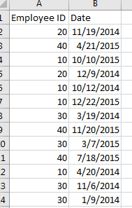
Looking at this data I may want to understand an which employees and when do they scan into a building over time. Breaking this down further I may want to review Q1 of 2014 to Q1 of 2015 to see if the employee’s attendance increased or decreased.
Here is the raw data we will be working with, Employee IDs Raw Data. Our first step is to Load this data into PowerBI. I have already generated the Advanced Editor query to load this file. You can use the following code to load the Employee ID data:
let
 Source = Csv.Document(File.Contents("C:\Users\Mike\Desktop\Employee IDs.csv"),[Delimiter=",", Columns=2, Encoding=1252, QuoteStyle=QuoteStyle.None]),
 #"Promoted Headers" = Table.PromoteHeaders(Source),
 #"Changed Type" = Table.TransformColumnTypes(#"Promoted Headers",{{"Employee ID", Int64.Type}, {"Date", type date}}),
 #"Sorted Rows1" = Table.Sort(#"Changed Type",{{"Date", Order.Ascending}}),
 #"Calculated Start of Month" = Table.TransformColumns(#"Sorted Rows1",{{"Date", Date.StartOfMonth, type date}}),
 #"Grouped Rows" = Table.Group(#"Calculated Start of Month", {"Date"}, {{"Scans", each List.Sum([Employee ID]), type number}})
in
 #"Grouped Rows"
Note: I have highlighted Mike in red because this is custom to my computer, thus, when you’re using this code you will want to change the file location for your computer. For this example I extracted the Employee ID.csv file to my desktop. For more help on using the advanced editor reference this tutorial on how to open the advance editor and change the code, located here.
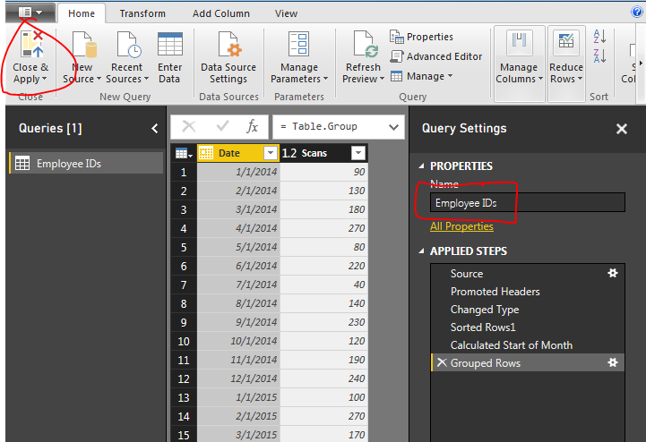
Next name the query Employee IDs, then Close & Apply on the Home ribbon to load the data.
Next we will build a series of measures that will calculate our time ranges which we will use to calculate our Percent Change (% Change) from month to month.
Now build the following measures:
Total Scans, sums up the total numbers of badge scans.
Total Scans = SUM('Employee IDs'[Scans])
Prior Month Scans, calculates the sum of all scans from the prior month. Note we use the PreviousMonth() DAX formula.
Prior Month Scans = CALCULATE([Total Scans], PREVIOUSMONTH('Employee IDs'[Date]))
Finally we calculate the % change between the actual month, and the previous month with the % Change measure.
% Change = DIVIDE([Total Scans], [Prior Month Scans], blank())-1
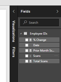
Completing the new measures your Fields list should look like the following:
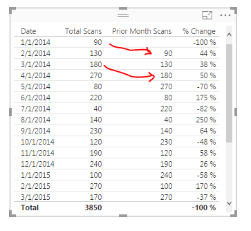
Now we are ready to build some visuals. First we will build a table like the following to show you how the data is being calculated in our measures.
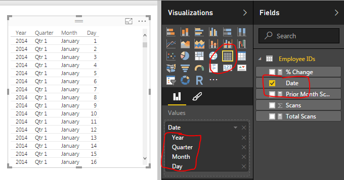
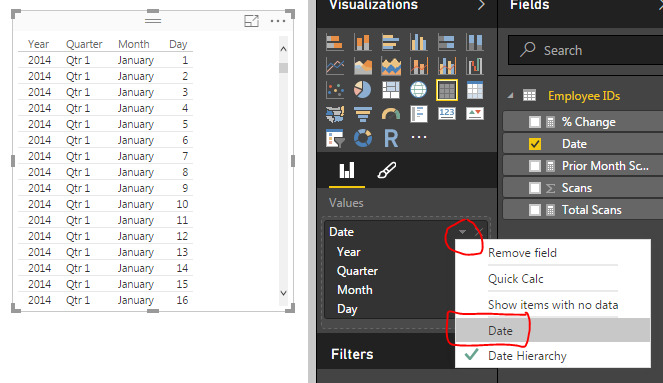
When we first add the Date field to the chart we have a list of dates by Year, Quarter, Month, and Day. This is not what we want. Rather we would like to just see the actual date values. To change this click the down arrow next to the field labeled Date and then select from the drop down the Date field. This will change the date field to be viewed as an actual date and not a date hierarchy.
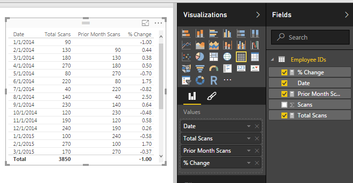
Now add the Total Scans, Prior Month Scans, and % Change measures. Your table should now look like the following:
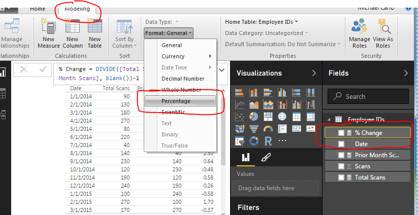
The column that has % Change does not look right, so highlight the measure called % Change and on the Modeling ribbon change the Format to Percentage.
Finally now note what is happening in the table with the counts totaled next to each other.
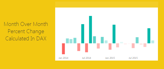
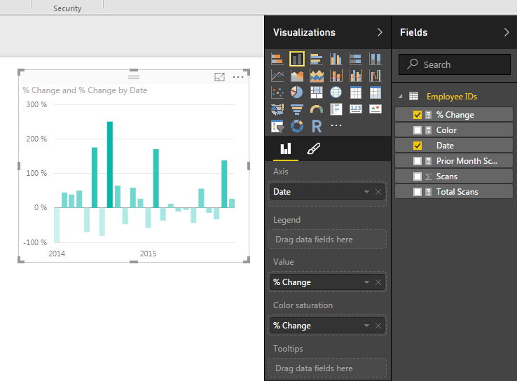
Now adding a Bar chart will yield the following. Add the proper fields to the visual. When your done your chart should look like the following:
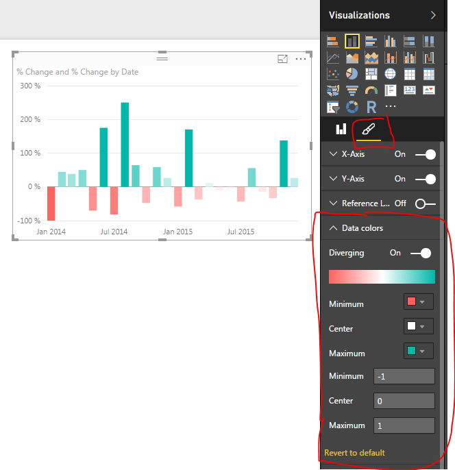
To add a bit of flair to the chart you can select the Properties button on the Visualizations pane. Open the Data Colors section change the minimum color to red, the maximum color to green and then type the numbers in the Min, Center and Max.
Well, that is it, Thanks for stopping by. Make sure to share if you like what you see. Till next week.
Want to learn more about PowerBI and Using DAX. Check out this great book from Rob Collie talking the power of DAX. The book covers topics applicable for both PowerBI and Power Pivot inside excel. I’ve personally read it and Rob has a great way of interjecting some fun humor while teaching you the essentials of DAX.