Tag: Advanced

  • All Columns have Data Types in DAX, Or do they?

    All Columns have Data Types in DAX, Or do they?

    To say this another way. Not all columns have datatypes in DAX, specifically speaking to using dynamic ranking with an “Other” category. Let me explain.

    The Tabular model is comprised of tables with typed columns. This is a truth learned in one’s Tabular infancy. Whether the table is imported, calculated, or Directly Queried does not matter; all tables have columns with explicitly defined types.

    DAX is the language of the Tabular model. It has less type discipline than tables in the Tabular model. Measures can have a Variant data typeImplicit type conversions abound. Nor are DAX expressions limited to returning scalar values. DAX is a query language. An expression may return a table. When defining a table in DAX, projected columns have no explicit type. Each row’s value is calculated independently and its type depends on its value. This is the phenomenon we seek to explore in this post. If this seems unsurprising, you can probably stop here.

    A practical scenario

    Here is the scenario where I discovered this. I was helping a colleague with a dynamic ranking measure and aggregation. The requirement read:

    Show the top for production plants as ranks 1 through 4. Group all others ranked 5 or lower together as “Other”.

    We have three tables:

    1. a fact table 'Fact'
    2. a dimension table 'Dim', related to 'Fact' with the relationship 'Fact'[DimKey] <-N:1- 'Dim'[DimKey]
    3. a disconnected table, 'Rank Selector', with the values: “1”, “2”, “3”, “4”, and “Other”.

    We aggregate 'Fact'[Value]. Here is a Power BI file with sample data and code.

    Our first try

    We started with a measure [Agg] as our base measure.

    Agg = SUM ( 'Fact'[Value] )

    [_Rank (variant)] is a helper ranking measure, returning a rank 1-4 or “Other”.

    _Rank (variant) =
    VAR rawRank = RANKX ( ALL ( 'Dim' ), [Agg],, DESC )
    // note this value is either a number 1-4 OR the string, "Other"
    VAR groupedRank = IF ( rawRank <= 4, rawRank, "Other" )
    RETURN
        groupedRank

    Below is a screengrab of these two measures evaluated against our 'Dim'[Plant]. As you can see, [Agg] returns a value for each plant. The top four plants have ranks of 1, 2, 3, and 4. The other plants all have the same rank, “Other”. This is all as expected.
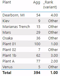
    'Dim'[Plant] with [Agg] and [_Rank (variant)] measures, working largely as expected. Each dim value has a value for [Agg] and a rank of 1-4 or the string, “Other”.

    The issue reared its head when we attempted to use these ranks to define a new visual based on 'Rank Selector'[Rank]. We defined a measure to show [Agg] based on the plant’s rank (1-4 or “Other”), rather than the plant name. Note that 'Rank Selector'[Rank] is a column in a data model table, with Data type: Text. Our expectation is that we will see a table like the image below.
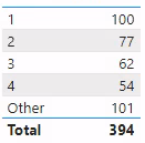
    A table visualization showing six rows with labels: “1”, “2”, “3”, “4”, “Other”, and “Total”; and showing an aggregate alongside each.

    Wherein our heroes encounter a challenge

    [Ranked Agg (variant)] is the display measure to show aggregations against 'Rank Selector'[Rank]. We wrote the variant version you see below first, not realizing the perils that laid ahead. (Correct implementations follow later.)

    Ranked Agg (variant) = 
    VAR rankContext = VALUES ( 'Rank Selector'[Rank] )
    VAR ranked =
        ADDCOLUMNS (
            ALL ( 'Dim' ),
            "@rank", [_Rank (variant)],
            "@val", [Agg]
        )
    VAR currentRank = FILTER ( ranked, [@rank] IN rankContext )
    VAR result = SUMX ( currentRank, [@val] )
    RETURN
        result

    When we visualize this measure against 'Rank Selector'[Rank], we get the result below.
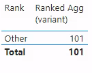
    A table visualization showing only the 'Rank Selector'[Rank] value “Other” and “Total”. Specifically, we do not see any value for ranks “1”, “2”, “3”, or “4”.

    A table visualization showing only the 'Rank Selector'[Rank] value “Other” and “Total”. Specifically, we do not see any value for ranks “1”, “2”, “3”, or “4”.

    What is going on here? We see data only for the Rank Selector'[Rank] label “Other” but none of the numbers. Let us walk through the measure step-by-step to understand this result.

    VAR rankContext = VALUES ( 'Rank Selector'[Rank] )

    rankContext captures whatever the current filter context is for 'Rank Selector'[Rank]. This is one or a collection of the values: “1”, “2”, “3”, “4”, and “Other”. For a detail row of a table visualization, the context contains exactly one of those values. For a total row (assuming no other slicers or filters), the context contains all of those values.

    VAR ranked =
        ADDCOLUMNS (
            ALL ( 'Dim' ),
            "@rank", [_Rank (variant)],
            "@val", [Agg]
        )

    ranked is a table with all rows and columns of the data model table 'Dim' and two projected columns, [@rank] and [@val]. For any row, i.e., for any specific plant, [@rank] is one of 1-4 or “Other”. Many rows may have [@rank] = "Other". We do not expect ties, so there are exactly four rows with numeric ranks, one each for the ranks 1-4. (This table looks like the first table visualization screenshot above.)

    The critical part of both the ranking logic and the phenomenon we are exploring is in currentRank. This is a subset of the table, ranked, holding only the row or rows which have a [@rank] value that exists in the filter context captured in rankContext (again, one or a collection of the values “1”, “2”, “3”, “4”, and “Other”).

    Note, that we see data only for the Rank Selector'[Rank] label “Other”. As you recall, our [_Rank (variant)] seemed to work correctly above – it definitely returned ranks 1-4, not just “Other”. 'Rank Selector'[Rank] has the correct values. We checked that our logic in [Ranked Agg (variant)] was correct. We verified in DAX Studio that ranked held the correct table. We even got to the point that we checked whether VALUES was behaving as we expected in rankContext. (I will note that if you find yourself verifying the behavior of an expression as basic as VALUES ( 'Rank Selector'[Rank] ), then you, too, may find yourself questioning what has brought you to this point.)

    VAR currentRank = FILTER ( ranked, [@rank] IN rankContext )

    We continued checking and troubleshooting and identified that currentRank had binary state: either it would be an empty table or it would be a table holding only rows with [@rank] values of “Other”. It would never hold a row with a rank value of 1, 2, 3, or 4. It seemed that the predicate in our FILTER would never find 1 to be equal to 1, or 2 equal to 2, and so on.

    How could basic logic be so broken just in this measure? There was much gnashing of teeth. Several head-shaped indents were beaten into the nearest wall.

    DAX, the language, has a more permissive type system than the Tabular model

    You may have observed some apparent inconsistency in my quoting or not-quoting the rank values above. In fact, I have been scrupulous to always quote values when referring to 'Rank Selector'[Rank], the model column with type Text, and to not-quote the rank values returned from [_Rank (variant)]. The column 'Rank Selector'[Rank] has exclusively string values. The measure [_Rank (variant)] sometimes returns a numerically typed value in the range 1-4 and sometimes returns the string “Other”.

    In DAX, 1 = 1 is an equality test that returns TRUE. Similarly, 1 IN {1, 2, 3, 4} returns TRUE, because 1 = 1 and 1 exists in the table there. In DAX, 1 = "1" is an equality test that throws a type error. Numbers cannot be tested for equality with strings. They are different types. Therefore, a number can never be equal to a string. Thus, 1 IN {"1", "2", "3", "4", "Other"} also throws a type error.

    The lightbulb moment

    In [Ranked Agg (variant)]currentRank has a column [@rank] with type Variant. Sometimes, [@rank] has a value in the range 1-4, type Whole Number. Sometimes it has the value “Other”, type Text. When we evaluate the predicate [@rank] IN rankContext, there are exactly two possible results. Either we ask for an impossible membership test, “Is this numerically typed rank value in the set of Text values?”, or we ask whether the string “Other” is in that set. The first cannot succeed. The second only succeeds for the “Other” rank.

    The Fix

    The fix, then, is straightforward. We must always return a value of type Text in our ranking measure. Correct measures are below with comments highlighting the modifications.

    _Rank (typed) = 
    VAR rawRank = RANKX ( ALL ( 'Dim' ), [Agg],, DESC )
    VAR groupedRank =
        // with an explicit typecast, our measure now *always* returns a string-typed value
        IF (
            rawRank <= 4,
            FORMAT ( rawRank, "0" ), // force string type
            "Other"
        )
    RETURN
        groupedRank
    
    Ranked Agg (typed) = 
    VAR rankContext = VALUES ( 'Rank Selector'[Rank] )
    VAR ranked =
        ADDCOLUMNS (
            ALL ( 'Dim' ),
            "@rank", [_Rank (typed)], // the only difference here is using our typed rank helper measure
            "@val", [Agg]
        )
    VAR currentRank = FILTER ( ranked, [@rank] IN rankContext )
    VAR result = SUMX ( currentRank, [@val] )
    RETURN
        result

    The measures above give us the results we expected all along, as you can see in the table visualization below.
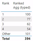
    A table visualization showing 6 rows with labels: “1”, “2”, “3”, “4”, “Other”, and “Total”; and showing the correct values of [Ranked Agg (typed)] alongside.

    Below is a screengrab of all the measures in visualizations, so you can see the differences.
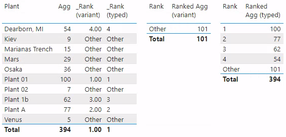
    A screenshot with all three of the table visualizations shown prior in this post: the 'Dim'[Plant] table with [Agg][_Rank (variant)], and [_Rank (typed)]; the incorrect behavior with [Ranked Agg (variant)]; and the correct behavior with [Ranked Agg (typed)].

    Summary

    Tabular model tables have columns of explicit type. DAX expressions have implicit types. Columns defined in DAX have Variant type. Each row has an implicit type based on its value. If such a column is a Calculated Column added to a data model table, then an explicit type must be assigned and all values in that column will be cast to that type at load time. When such a column is used as an intermediate step in some calculation, each row may have a different type. If your operations depend on types, you must account for this explicitly. This is especially relevant when operating on data model and DAX tables together.

    Insights from the community

    When talking about this with some peers, Maxim Zelensky (blogTwitter) observed that there is no type indication in Power BI Desktop. Nevertheless, you can identify this sort of thing in DAX Studio. The result of a query such as that below will right-align Variant-typed values and left-align Text-typed values. This query references the included Power BI file and its results are shown in a screenshot below. You can observe similar alignment in the table visual shown above. In general, when visualized, numeric data is presented with right-alignment and textual data left-aligned. This practice predates Power BI; it is a general rule that Power BI and DAX Studio wisely adopted.

    EVALUATE
    ADDCOLUMNS (
        VALUES ( 'Dim'[Plant] ),
        "@text", [_Rank (typed)],
        "@variant", [_Rank (variant)]
    )
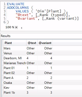
    A screenshot showing the results of the above query, with [@text] left-aligned and [@variant] right-aligned.

    Using the sample code and PBIX

    Here is a link to download the PBIX that was used for examples above. This has four visuals to demonstrate the phenomenon discussed in this blog post. The first visual is a table with 'Dim'[Plant][Agg][_Rank (variant)], and [_Rank (typed)]. Of note in the first visual is left-vs-right alignment of the two [_Rank ...] measures. The second visual is a table with 'Rank Selector'[Rank] and [Ranked Agg (variant)], showing the incorrect results of the measure depending on a Variant-typed intermediate column, with a value only for rank “Other”. The third visual contrasts with the second, using [Ranked Agg (typed)] to show the correct behavior of the dynamic ranking and grouping logic, with a value for all ranks and a correct total. Lest one protest that the phenomenon above may be an artifact of using VARs, the last visual, on the bottom, shows an example that uses no VARs and references no other measures. The behavior of this last visual is identical to the incorrect [Ranked Agg (variant)] version.

  • Introducing Lingo

    Introducing Lingo

    Update: This tool has been deprecated as of 2024-11-27. You can now find this as a downloadable HTML file at the following Github page.

    In April of 2018 the Microsoft team released the ability to edit the Linguistic schema in Power BI desktop.  For those who are not aware of the linguistics, essentially, this is the code that drives how Power BI can interpret your data model when you use Q & A.  The linguistic schema is defining how the computer is able to figure out the best visual relating to your question.  In Power BI desktop you can double click on the white space of a report page and then the Q & A prompt appears.  Then type a statement into the Q & A box, this in turn generates a visual.

    In both the Desktop program and in the PowerBI.com service, Q & A is an impressive feature.  By default the Power BI desktop creates a linguistics schema about the data model.  However, there are some details that the linguistics schema can’t detect.  This is where you come in.  In the Power BI Desktop you can download the Linguistics file, make any number of changes or additions to the file and then re-upload the file back to Power BI Desktop.  But, there is a slight catch.  The downloaded files can be quite large and a little difficult to navigate.  PowerBI.Tips to the rescue.

    Introducing Lingo, the free linguistics code editor.Introducing Lingo

    Lingo is a web app that allows you to upload your linguistics schema into an easy to use editor.  It includes search, code validation, and code blocks that you can use to make writing code easier.  Check out the video below to see how it works:

    For the full details on the linguistics schema visit the following article from Microsoft.  A sample Power BI file, Linguistics model, and Linguistics Spec can be downloaded here.  Well that about wraps it up, thanks for reading and happy coding.

    If you like what you learned about today and want to stay updated, please follow me on Twitter, Linkedin, and YouTube for the latest updates.

  • Crazy Table Gymnastics – Part 2 – Build Support Materials

    Crazy Table Gymnastics – Part 2 – Build Support Materials

    This is part 2 in the 3 part series on developing super cool tables using some fancy measures.  In part 1 we walked through how to build a table that uses an un-pivoted data source in the Query Editor.  This technique allows you to change the types of categorical values in a table.  If you missed part 1 and want to get caught up follow this link.  Now, continuing with the series, Part 2, we will build the supporting materials (Selector Table, What If Slicers, and measures) for the report.

    Once we are done the final product will look like the following:

    Part 2… Go.

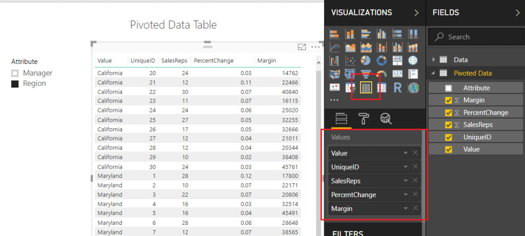
    To make sure we are starting off on the correct step.  We left off part 1 when we had completed a Pivoted Data Table and included an Attribute Slicer that would allow us to toggle between the Manager and Region Categories.  Your table should look like the following diagram:  (If you don’t have this you might want to start with Part 1 found here)

    Pivoted Data Table
    Pivoted Data Table

    Note: I have also included a Slicer which is used with the Attribute field.

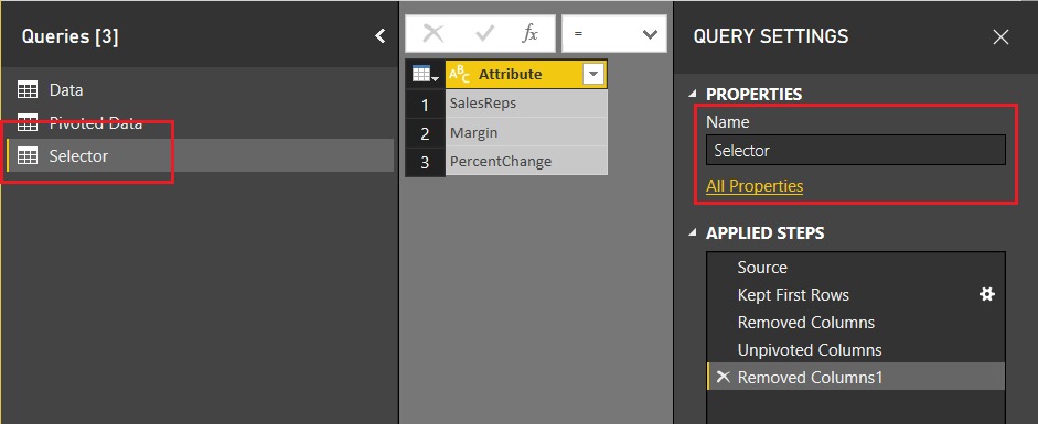
    Next, we will need to add a table that will allow us to use the SalesReps, PercentChange, and Margin column headers in our report.  On the Home ribbon click Edit Queries, then select New Source on the Home ribbon.  In the Get Data window select Blank Query, click Connect to proceed.  Open the advanced editor by clicking the Advanced Editor button found on the Home ribbon.  Enter the following M code into the Advanced Editor:

    let
       Source = #"Pivoted Data",
       #"Kept First Rows" = Table.FirstN(Source,1),
       #"Removed Columns" = Table.RemoveColumns(#"Kept First Rows",{"Attribute", "Value", "UniqueID"}),
       #"Unpivoted Columns" = Table.UnpivotOtherColumns(#"Removed Columns", {}, "Attribute", "Value"),
       #"Removed Columns1" = Table.RemoveColumns(#"Unpivoted Columns",{"Value"})
    in
       #"Removed Columns1"

    Click Done to close the Advanced Editor.  Rename the table to Selector.  When you are finished your table should look like the following:

    Create Selector Table
    Create Selector Table

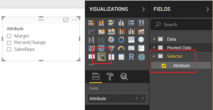
    Click Close & Apply on the Home ribbon to close the Query Editor.  Add a slicer with the following selections:

    Add Selector Attribute Slicer
    Add Selector Attribute Slicer

    Now, we want to detect which of the Attributes have been selected from this table.  We can accomplish this by creating a measure using the DAX function SELECTEDVALUE.  Right Click on the table named Selector and from the drop down select New Measure.  Enter the following DAX equation:

    rankBy = SELECTEDVALUE(Selector[Attribute])

    In addition to the knowledge of which column was selected from the selector table, we will also want to detect to make sure at least one categorical value has been selected.  The categorical values we are talking about were generated earlier.  The values could be either the Manager or Region values of the Attribute column in the Pivoted Data table.  Using the ISFILTERED DAX function enables this section.  Add the following measure to the Pivoted Data table:

    Attribute Filtered = ISFILTERED('Pivoted Data'[Attribute])

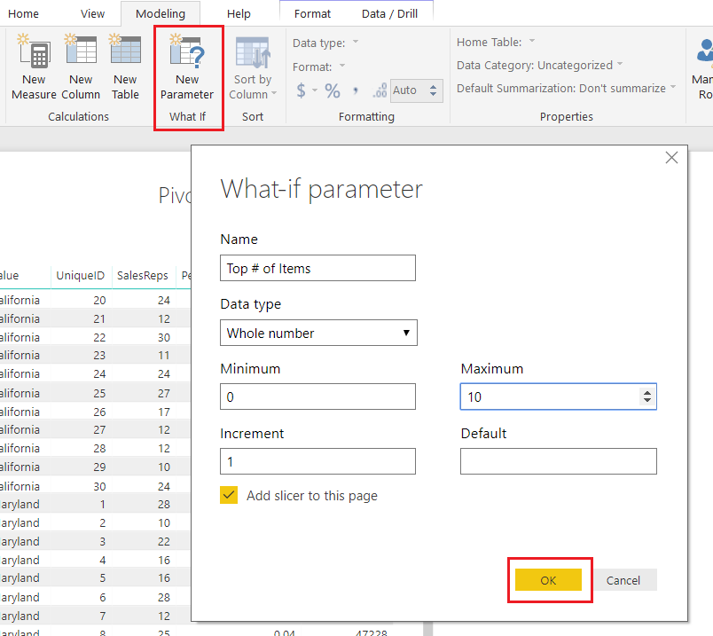
    Next, we need to gather some user input in the form of a number from 1 to 10.  To input this information we need to produce a What If Parameter.  On the Modeling ribbon click New Parameter in the What If section of the ribbon.  Enter the following information into the What-if parameter dialog box:

    What If Parameter
    What If Parameter

    Note: Don’t forget to change the Name of the parameter.

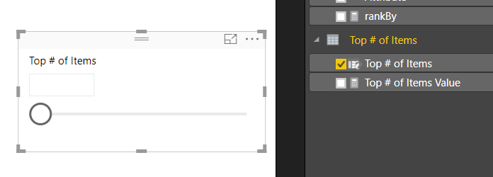
    Click OK to proceed.  Power BI will automatically produce a measure table, a measure and a slicer on the report page.

    Slicer Produced by What-if
    Slicer Produced by What-if

    Note: By default there is nothing selected in the box.  However, you can adjust the slicer and a number will appear within the value box.  You can also type in a number between 1 and 10 to the box to adjust the value.

    This is where we go crazy with DAX.  This portion of DAX is where all the magic happens.

    We start off by building our totals measures.  Place all these measures in the Pivoted Data table.

    Total % Change = MAX( 'Pivoted Data'[PercentChange] )
    Total Margin = SUM( 'Pivoted Data'[Margin] )
    Total SalesReps = SUM( 'Pivoted Data'[SalesReps] )

    These will be used repeatedly in our next group of DAX formulas.

    The following measures will produce a calculated ranking for each numerical column.  OK, Pause, This part really excites me here because the next few measures are where the magic happens.  Pay close attention to what is happening here.  Un-Pause, by using the DAX Switch function we can dynamically tell Power BI to adjust which column we want to see ranked by the top items.  For example, if we select SalesReps in our attribute slicer.  The following measures will automatically rank all the items in the table by the column named SalesReps.  Thus, the items with the highest counts of SalesReps will be listed first.  When you select Margin, the table will automatically adjust and re-rank the items by the Margin column.  This is being done in the switch statement.  For each column we are calculating custom rankings and then hiding or replacing values with the Blank() DAX function to not show items we don’t want.

    Enter the following three measures into the Pivoted Data Table:

    Rank Margin = if( [Attribute Filtered],
        SWITCH( [rankBy]
            ,"Margin", CALCULATE( [Total Margin], FILTER('Pivoted Data', RANKX( ALLEXCEPT('Pivoted Data','Pivoted Data'[Value]), [Total Margin]) <= [Top # of Items Value]) )
            ,"PercentChange", CALCULATE( [Total Margin], FILTER('Pivoted Data', RANKX( ALLEXCEPT('Pivoted Data','Pivoted Data'[Value]), [Total % Change]) <= [Top # of Items Value]))
            ,"SalesReps", CALCULATE( [Total Margin], FILTER('Pivoted Data', RANKX( ALLEXCEPT('Pivoted Data','Pivoted Data'[Value]),[Total SalesReps]) <= [Top # of Items Value]))
        )
        , BLANK() )
    
    Rank PercentChange = if( [Attribute Filtered],
         SWITCH( [rankBy],
           "PercentChange", CALCULATE( [Total % Change], FILTER('Pivoted Data', RANKX( ALLEXCEPT('Pivoted Data','Pivoted Data'[Value]), [Total % Change]) <= [Top # of Items Value]))
           ,"Margin", CALCULATE( [Total % Change], FILTER('Pivoted Data', RANKX( ALLEXCEPT('Pivoted Data','Pivoted Data'[Value]), [Total Margin]) <= [Top # of Items Value]))
           ,"SalesReps", CALCULATE( [Total % Change], FILTER('Pivoted Data', RANKX( ALLEXCEPT('Pivoted Data','Pivoted Data'[Value]), [Total SalesReps]) <= [Top # of Items Value]))
        )
        , BLANK() )
    
    Rank SalesReps = if( [Attribute Filtered],
        SWITCH( [rankBy]
            ,"SalesReps", CALCULATE( [Total SalesReps], FILTER('Pivoted Data', RANKX( ALLEXCEPT('Pivoted Data','Pivoted Data'[Value]), [Total SalesReps]) <= [Top # of Items Value]))
            ,"Margin", CALCULATE( [Total SalesReps], FILTER('Pivoted Data', RANKX( ALLEXCEPT('Pivoted Data','Pivoted Data'[Value]), [Total Margin]) <= [Top # of Items Value]))
            ,"PercentChange", CALCULATE( [Total SalesReps], FILTER('Pivoted Data', RANKX( ALLEXCEPT('Pivoted Data','Pivoted Data'[Value]), [Total % Change]) <= [Top # of Items Value]))
        )
        , BLANK() )

    Whew, that was a ton of measures.  All the key components are complete now.  In part 3 we will clean up our report page and make it shine.  I hope you enjoyed this tutorial. Also, follow me on Twitter and Linkedin where I will post all the announcements for new tutorials and content.

    Linkedin Twitter
  • Crazy Table Gymnastics – Part 1 – Dynamic Column Categories

    Crazy Table Gymnastics – Part 1 – Dynamic Column Categories

    When I teach Power BI to new users, there are typically questions about how to get Power BI to act more like Pivot Tables in Excel.  Through my discussions, two key pieces of functionality stand out to me that people want.

    1. They would like to select a categorical property to adjust the table.  In this scenario a user would want to select the State, Sales Territory, or something else that describes a breakdown of the data.  This is similar to adding a field of data into the Rows selection for Pivot Tables.
    2. They want the ability to rank a column and select only the top N number of items in a given column.  Imagine that you have Sales Units, Revenue, or some other numerical column.  Then based on a selected column such as Sales Units, I want to see the top 3 or 4 sales items.  This would be a similar in the excel experience when you modify the filters for a given pivot table column.

    Disclaimer: This is quite a large topic and therefore I have broken this up into three segments for read-ability.  Thus, to poke your curiosity below is the final example of the report.  We will walk through reach phase of this report, so you can produce this dynamic table. 

    This series of blogs will be broken up into three parts.

    Part 1: Build a Table or Matrix visual that can dynamically change based on a slicer

    Part 2: Build supporting tables & measures

    Part 3: Bring it all together for the final report

    OK, hold on tight, here we go!

    Let’s begin with acquiring our data.  Open Power BI Desktop.  Click Get Data on the Home ribbon and select Excel.  When the Open dialog box opens enter the following file name, and click Open:

    https://powerbitips.blob.core.windows.net/powerbitipsdatas/SampleData.xlsx

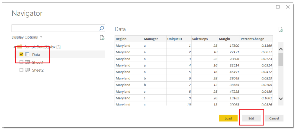
    The Navigator window will open showing you the contents of the file.  Select the Data Table by clicking in the square next to the word labeled Data, click Edit to load the data and enter the Query Editor.

    Load Data from Excel
    Load Data from Excel

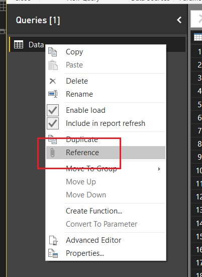
    Next, Right Click on the table labeled Data in the Queries pane, from the drop-down menu select Reference.

    Create Reference Query
    Create Reference Query

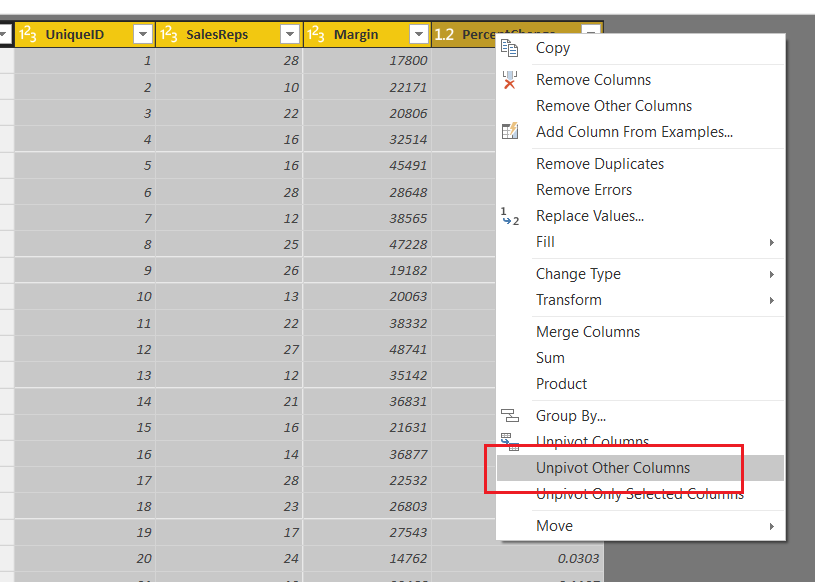
    This will produce a second table labeled Data (2).  In the Properties pane on the right side of the screen edit the name of the query to Pivoted Data. Select the columns UniqueID, SalesReps, Margin, and PercentChange by holding Ctrl and clicking on each column.  While keeping all four (4) columns selected right click on the last column and select Unpivot Other Columns.

    Unpivot Columns
    Unpivot Columns

    Note: It is important to notice that we selected Unpivot Other Columns instead of selecting the Region and Manager columns and selected Unpivot Columns.  Selecting Region and Manager and selecting Unpivot Columns will achieve the same results, but if our excel file or underlying data set adds more Categorical columns our query will break.  Using this technique creates a flexible query that can handle any number of new categorical columns.  You know your data the best, and how it will change over time.  It is important to consider these aspects when loading data via the Query Editor. 

    We have completed our data load.  On the Home ribbon click Close & Apply to complete the data load for our two tables, Data and Pivoted Data.

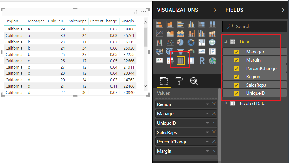
    Load the Fields from the Data table into a Table Visual, as shown below:

    Data Fields Loaded Into Table
    Data Fields Loaded Into Table

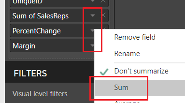
    For the following fields SalesReps, PercentChange, and Margin change the Fields to SUM by clicking on the Triangle next to each field’s name.  We will use this information to confirm that our Pivoted table is providing the correct data.

    Change Fields to Sum
    Change Fields to Sum

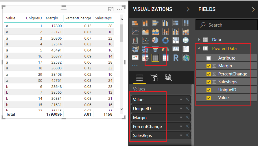
    Add a second Table visual and bring over the fields from the second data set, our Pivoted Data table.  Be sure to leave off the Attribute column as this will not be needed in this second table.

    Table for Pivoted Data
    Table for Pivoted Data

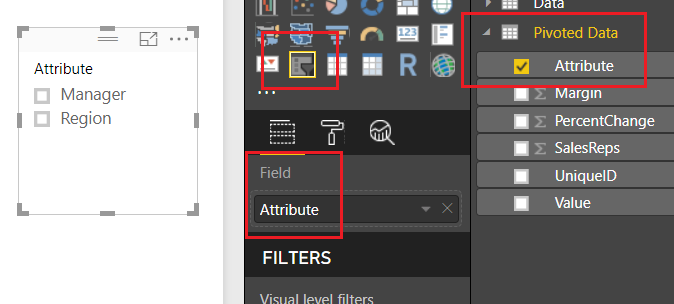
    Add a Slicer to the report layout and add the column labeled Attribute from the Pivoted Data table.

    Add Slicer
    Add Slicer

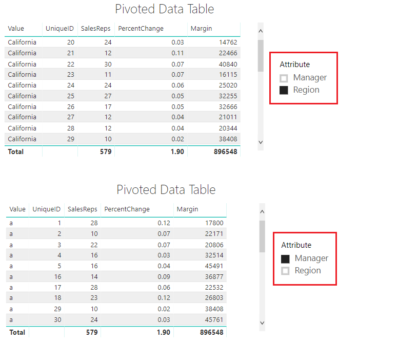
    Notice we now have the ability to select either the Manager Column or the Region column.  By doing so, we are able to change the columns within our table to only show the items relevant to our slicer selection.  Pretty cool.

    Using The Slicer
    Using The Slicer

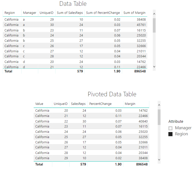
    It’s also important to note here that in our Pivoted Data Table, we can only acquire the correct totals with a single attribute selected.  When the slicer has no selection our totals for SalesReps, PercentChange and Margin are all twice the amount they should be.  Later on, in part 2 of this tutorial, we will fix this using measures.

    Data In Both Tables Match
    Data In Both Tables Match

    Thanks for reading along.  Stay tuned for part 2 where we will build supporting data tables to aid the user experience on the report page.  If you like what you learned, please forward this on to someone else who would enjoy these free tutorials.  Also, follow me on Twitter and Linkedin where I will post all the announcements for new tutorials and content.

    Linkedin Twitter
  • Creating A DAX Calendar

    Creating A DAX Calendar

    There are many cases when you will need to create a date table within Power BI desktop.  This could be as simple as creating a master date table or more complex such as creating a monthly or weekly index number tied to a date.  To create a date table there are two methods for creating a date table.  Method one, create the table directly in the Power BI Desktop, or method two load the date table from the data source.

    For this tutorial we will walk through a couple different examples that are specifically addressing creating a date calendar via DAX expressions.

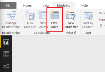
    Let’s begin by making a basic table.  Open Power BI Desktop, on the Modeling ribbon click New Table.

    New Table
    New Table

    In the formula bar enter the following DAX expression:

    Dates  = 
      GENERATE ( 
        CALENDAR ( DATE ( 2017, 1, 1 ), DATE ( 2017, 12, 31 ) ), 
        VAR currentDay = [Date]
        VAR day = DAY( currentDay )
        VAR month =  MONTH ( currentDay ) 
        VAR year =  YEAR ( currentDay )
      RETURN   ROW ( 
        "day", day, 
        "month", month, 
        "year", year )
      )

    This generates a simple date table.  Let’s walk through what is happening here.

    1. The CALENDAR DAX function generates a table with a list of dates from Jan 1 to Dec 31 of 2017.
    2. We define variables (denoted by VAR) to capture details from the column named [Date] that is created by the CALENDAR function.
    3. The Return function generates one row at a time.  The row iterates through each [Date] item in the list which was created by the CALENDAR function.  Variables are re-calculated for every row execution.

    Note: When creating DAX tables as we are doing so in this example, the DAX table only refreshes when the report refreshes.  Thus, if you want the date list to increase over time, or your using a NOW() in the DAX table you will need to be sure to schedule refreshes for the Power BI report in the PowerBI.com service.

    By contrast we can also generate the same data table by calculating our data column by column.  Again, on the Modeling ribbon click the New Table icon and add the following DAX:

    Dates 2 = ADDCOLUMNS(
      CALENDAR( DATE( 2017, 1, 1) , DATE(2017, 12, 31) ), 
      "day", DAY([Date]), 
      "month", MONTH([Date]), 
      "year", YEAR([Date])
      )

    While this is great, we have a date table now, but what we lack is flexibility and automatic time intelligence.  One option to change this table to auto detect dates within your data model is to replace the CALENDAR DAX statement with CALENDARAUTO().

    To use CALENDARAUTO we need to supply a table with a column of dates.  We will quickly create a dummy data table with a couple of dates, so we can use CALENDARAUTIO.

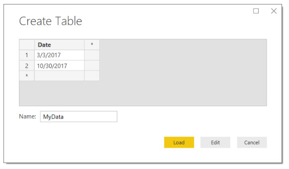
    Click Enter Data on the Home ribbon.  Enter the following information into the Create Table screen.  Click Load to add this data to the data model.

    Enter Date Table
    Enter Date Table

    Now that we have loaded a table into the model with two dates, we can add our new date table.  On the Modeling ribbon click the New Table icon and add the following DAX:

    Dates 3 =
      GENERATE (
        CALENDARAUTO(),
        VAR currentDay = [Date]
        VAR day = DAY( currentDay )
        VAR month =  MONTH ( currentDay )
        VAR year =  YEAR ( currentDay )
      RETURN  ROW ( 
        "day", day,
        "month", month,
        "year", year )
      )

    Note: In the MyData table we added two dates, 3/3/2017 and 10/30/2017.   When we look at the included dates in the new Date 3 table we have every date listed from January 1 to December 31st.  This is because the DAX function CALENDARAUTO will return the entire year of calendar dates even if it only finds one date within a given year period of time.  

    Let’s say we want to build a date calendar that will automatically grow and change over time.  We want to identify today’s date and then create a list of dates for the previous year.

    Moving back to generating a date table by rows we can now use the DAX NOW function.  On the Modeling ribbon click the New Table icon and add the following DAX:

    Dates 4  =
      GENERATE (
        CALENDAR( DATE( YEAR( NOW() ) - 1, MONTH( NOW() ), DAY( NOW()) ), NOW()),
        VAR currentDay = [Date]
        VAR day = DAY( currentDay )
        VAR month = MONTH ( currentDay )
        VAR year = YEAR ( currentDay )
      RETURN ROW (
        "day", day,
        "month", month,
        "year", year )
     )

    Note: In this DAX table we used the NOW() function which returns a date and time.  The same can be done when using the TODAY() function which only returns the date and not the time.

    This now generates is a date table that starts one year ago and populates all the dates until today.  For example, if today is 10-29-2017, then the date list would start at 10-29-2016 and end on 10-29-2017.  Pretty cool…

    Let us move further down the rabbit hole.  We can also start adding calculations that helps us move through date time calculations.  For example, you may want to calculate this month’s total sales and possibly last month’s sales.  By adding columns with an index, you can quickly shift time periods.  Doing so makes time calculations much easier.

    On the Modeling ribbon click the New Table icon and add the following DAX:

    Dates 5 =
      GENERATE (
        CALENDAR( DATE( YEAR( TODAY() ) - 2, MONTH( TODAY() ), DAY( TODAY()) ), TODAY()),
        VAR startOfWeek = 1 // Where 1 is Sunday and 7 is Saturday, thus a 3 would be Tuesday    
        VAR currentDay = [Date]
        VAR days = DAY( currentDay )
        VAR months = MONTH ( currentDay )
        VAR years = YEAR ( currentDay )
        VAR nowYear = YEAR( TODAY() )
        VAR nowMonth = MONTH( TODAY() )
        VAR dayIndex = DATEDIFF( currentDay, TODAY(), DAY) * -1
        VAR todayNum = WEEKDAY( TODAY() )
        VAR weekIndex = INT( ROUNDDOWN( ( dayIndex + -1 * IF( todayNum + startOfWeek <= 6, todayNum + startOfWeek, todayNum + startOfWeek - 7 )) / 7, 0 ) )
      RETURN ROW (
        "day", days,
        "month", months,
        "year", years,
        "day index", dayIndex,
        "week index", weekIndex,
        "month index", INT( (years - nowYear ) * 12 + months - nowMonth ),
        "year index", INT( years - nowYear )
      )
    )

    Note: The DAX equation above will work in your report without any changes.  However, I made a variable called startOfWeek.  This variable allows you to define the start day of the week.  For example, if you data starts a new week on Sunday, then the startOfWeek number will be a 1.  If your data start of week begins on Wednesday then the start of week number would be a 4.  This allows you to auto detect the day of the week and then automatically arranges all your weekly index numbers in the correct format.  Try playing around with this variable to see how DAX table changes.

    So why work so hard on the date table?  Well by having a robust date table you can simplify many of your measures that you need to build for your report.  Consider the following example:

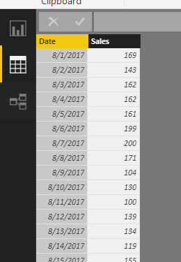
    You have a Sales table with a date and sales column.

    Sample Sales Data
    Sample Sales Data

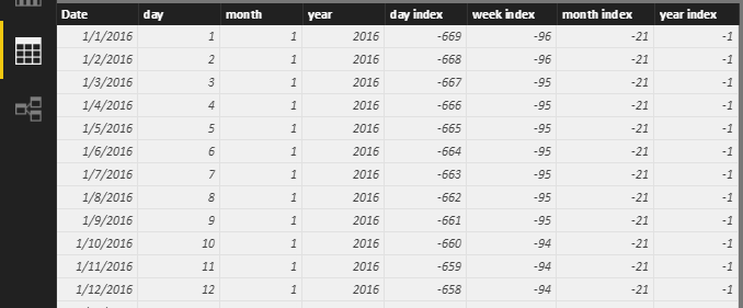
    And you have our fancy Dates 5 Table we created earlier:

    Date 5 Calendar
    Date 5 Calendar

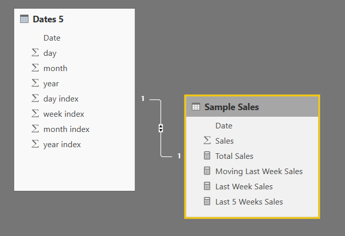
    The Date 5 table is linked to the Sample Sales table:

    Date and Sales Tables Linked
    Date and Sales Tables Linked

    You can now build the following DAX measures inside the Sample Sales table:

    Total Sales = SUM( 'Sample Sales'[Sales] )

    and

    Last Week Sales = CALCULATE( [Total Sales],  ALL('Dates 5'),  'Dates 5'[week index] = -1 )

    If you want to calculate something crazy like the last 5 weeks of sales you can calculate the following:

    Last 5 Weeks Sales = CALCULATE( [Total Sales], ALL( 'Dates 5' ),  AND( 'Dates 5'[week index]  <= -1,  'Dates 5'[week index] >= -5 ) )

    The nice thing about these measures is that every time the data set refreshes the dates will automatically recalculate the last week and last five weeks.

    If you want to be able to handle the additional filter context of the visual, you can pick up the visual filter context using variables (VAR).  Then you can RETURN a calculate function that will shift all your time ranges for you.

    Moving Last Week Sales = 
    VAR filterTime = SELECTEDVALUE('Dates 5'[week index], BLANK())
    RETURN CALCULATE( [Total Sales],  ALL( 'Dates 5'[Date] ), 'Dates 5'[week index] = filterTime - 1 )

    Same goes for a moving sum of the last five weeks of sales.

    Moving Last 5 Weeks Sales = 
    VAR filterTime = SELECTEDVALUE('Dates 5'[week index], BLANK())
    RETURN CALCULATE([Total Sales], ALL('Dates 5'[Date]), AND( 'Dates 5'[week index] <= filterTime -1, 'Dates 5'[week index] >= filterTime -5 ) )

    Well that is about it.  Thanks for following along.

    I am so thankful you have taken the time to read my tutorial.  My hope is that by using these free tutorials you can become a rock-star at work.  In order to keep these tutorials free please consider purchasing the Power BI Desktop file for this tutorial.  Come on it’s only a dollar, I mean you spent than that on your coffee this morning.

    You can pay with your PayPal account or via credit card

    [products limit = “1” columns=”4″ id=”12754″ ]

  • Power BI World Tour 2017 – Chicago – Top Tips

    Power BI World Tour 2017 – Chicago – Top Tips

    To everyone who was able to attend the Power BI World Tour 2017, Thank you!  It has been a pleasure presenting my favorite tips and trips.  This post consolidates all the links for each topic that was discussed.  All the links to the content are below, if you want to go through the tutorials at your own pace hit a link below.   When going through 7 topics in an hour, it is difficult to completely learn everything.  So, if your like me, you learn by doing, making mistakes and gritting it out until you understand.  Enjoy and have fun.

    Mike Carlo

    https://powerbi.tips/2016/06/loading-data-from-folder/

    https://powerbi.tips/2017/03/using-parameters-to-enable-sharing/

    https://powerbi.tips/2016/07/measures-month-to-month-percent-change/

    Note: Percent change seems like a major topic, if you want to see more tutorials on percent change you can follow this link for more tutorials.

    https://powerbi.tips/2016/04/power-bi-histogram-with-bins/

    https://powerbi.tips/2016/09/hexbin-plot-using-r/

    https://powerbi.tips/tools/report-theme-generator-v3/

    https://powerbi.tips/2017/08/best-practices-for-sharing/

    If you like this content and found it valuable make sure you share it with others.  Odds are they will like it as well.

    Want to meet more people who love Power BI, get connected with the Power BI User Groups (PUG).  Click this link to find your nearest PUG group.

  • Santa Loves Power BI and R

    Santa Loves Power BI and R

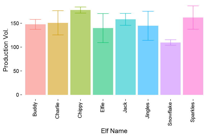
    This past week I was talking with the big guy up north, jolly old fella, and the discussion came up about his toy production levels.  Santa was complaining about how hard it was to measure the performance of all his elves.  Naturally I started babbling about how much I enjoy Power BI and that I use it on all kinds of sources of data, google analytics, excel sheets, sharepoint, and SQL data warehouses just to name a few.  Now by this point most people would have wandered off looking for another conversation, but I must have struck a chord with Santa.  He jumped right in the conversation and told me how he had just moved all his local data centers into Azure and more specifically SQL data warehouses.  It was saving him loads of money in addition it has freed up all his I.T. elves to move to more important tasks, building the NES Classic for Nintendo, they are way behind in production.  To make a long story longer, I was able to convince Santa to give me a small sample of data so I could show him how to use R to visualize his data in PowerBI.  Here is what I came up with:

    Santa Production Levels
    Santa Production Levels

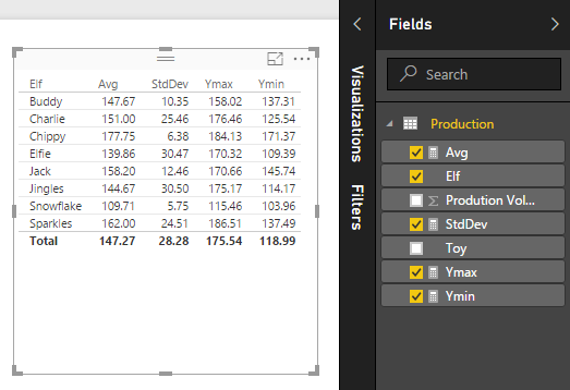
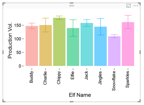
    Needless to say he was very pleased.  I explained the chart to Santa, each bar represents the average production volume for each elf.  Then the whiskers at the end of the bar represent the +1 and -1 standard deviation away from that mean.  It essentially tells you how consistent each elf is able to produce products and what is the average production rate.  For example, Buddy the Elf can produce an average 148 items in a day, he has a daily variance of 10 items.  Charlie can produce on average more items but has a wider daily variance.  Snowflake has the lowest average production level but is one of the more consistent producers.  Santa gave me a big smile and said “nice job.”

    Let’s walk through how I did this.

    Open up PowerBI Desktop, Click the Get Data button on the Home ribbon and select Blank Query.  Click Connect to open the Query Editor.  Click Advanced Editor on the View ribbon.  While in the Advanced Editor paste the following code into the editor window, click Done to complete the data load.

    Note: If you need some more help loading the data follow this tutorial about loading data using the Advanced Query Editor.  This tutorial teaches you how to copy and paste M code into the Advanced Editor.

    let
        Source = Excel.Workbook(Web.Contents("https://powerbitips03.blob.core.windows.net/blobpowerbitips03/wp-content/uploads/2016/12/Santa-Production.xlsx"), null, true),
        Production_Table = Source{[Item="Production",Kind="Table"]}[Data],
        #"Changed Type" = Table.TransformColumnTypes(Production_Table,{{"Elf", type text}, {"Toy", type text}, {"Prodution Volume", Int64.Type}})
    in
        #"Changed Type"

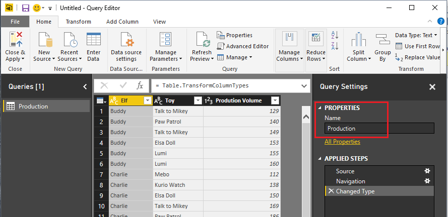
    Before you exit the query editor Rename the query to Production. It should look similar to the following:

    Production Query
    Production Query

    Click Close & Apply on the home ribbon.

    Add the following measures by click on the New Measure button on the Home ribbon.

    Avg = AVERAGE(Production[Prodution Volume])

    The Avg measure will determine the height of each bar in the bar chart.

    StdDev = STDEV.P('Production'[Prodution Volume])

    The StdDev will calculate the standard deviation for each elf.

    Ymax = [Avg]+ [StdDev]

    The Ymax calculation adds the Avg measure value to the standard deviation for production.  This produces the upper arm of the whisker.

    Ymin = [Avg]-[StdDev]

    The Ymin calculation is subtracts the standard deviation from the Avg measure value.  This produces the lower arm of the whisker.

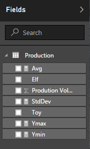
    Once you have completed making all the measures you should have a Production table with the following fields:

    Added Measures
    Added Measures

    Add the table visual by click on the Table visual in the Visualizations pane.  Add the Fields which are shown below.  Your table should look identical to this:

    Production Table
    Production Table

    Next, add the R Visual from the visualization Pane.  When you click on this you will get a message stating “Enable Script Visuals” click Enable to proceed.

    Note: If you have not installed R or enabled the preview features of R in Power BI you should follow this tutorial which helps you get everything set up.  For this particular visual we are using ggplot2.  This is a package for R and should be installed in the R environment.  You can follow this tutorial on how to install ggplot2.

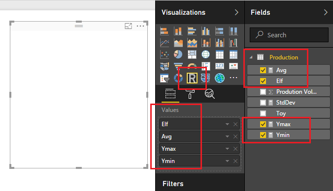
    Add the following fields into the R visual:

    Add Fields to R Visual
    Add Fields to R Visual

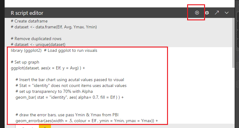
    Next in the R Script Editor add the following code to generate the R Script.

    library (ggplot2) # Load ggplot to run visuals

    # Set up graph
    ggplot(dataset, aes(x = Elf, y = Avg) ) +

    # Insert the bar chart using acutal values passed to visual
    # Stat = “identity” does not count items uses actual values
    # set up transparency to 70% with Alpha
    geom_bar( stat = “identity”, aes( alpha= 0.7, fill = Elf ) ) +
    # draw the error bars, use pass Ymin & Ymax from PBI
    geom_errorbar(aes(width = .5, colour = Elf , ymin = Ymin, ymax = Ymax)) +

    # Change the Labels
    labs(x = “Elf Name”, y = “Production Vol.” ) +

    # Make the theme simple and remove gridlines
    # Change the font size to 14
    theme_classic( base_size = 18 ) +

    # Remove the legend
    theme( legend.position = “none”) +

    # Change elements of the Axis, Angle, horizontal & Vertical position
    theme( axis.text.x = element_text(angle = 90, hjust = 1, vjust = 0.3),
    axis.text = element_text(colour = “black”),
    axis.ticks = element_line(colour = “black”),
    axis.title = element_text(colour = “black”),
    plot.background = element_rect(colour = NA) )

    Note: This code uses the R package ggplot2.  It will error out if you don’t have ggplot2 installed. 

    Click the run icon to execute the R script.

    Add R Script
    Add R Script & Run Script

    When the script runs you will have a beautiful production chart.

    R Chart
    R Chart

    Thanks for following along.  Like always be sure to share if you liked this content.  I am always, looking for feedback and possible topics so make sure you leave a comment below.

    If you want to download a similar example already completed you can download this example from the R Script Showcase (don’t forget to give me a thumbs up).

    Merry Christmas!

  • Measures – Year Over Year Percent Change

    Measures – Year Over Year Percent Change

    This tutorial is a variation on the month to month percent change tutorial.  This specific exploration in year over year performance was born out of reviewing my google analytics information.  The specific analysis question I am trying to answer is, how did this current month of website visitors compare to the same month last year.  For example I want to compare the number of visitors for November 2016 to November 2015.  Did I have more users this year in this month or last year?  What was my percent changed between the two months?

    Here is a sample of the analysis:

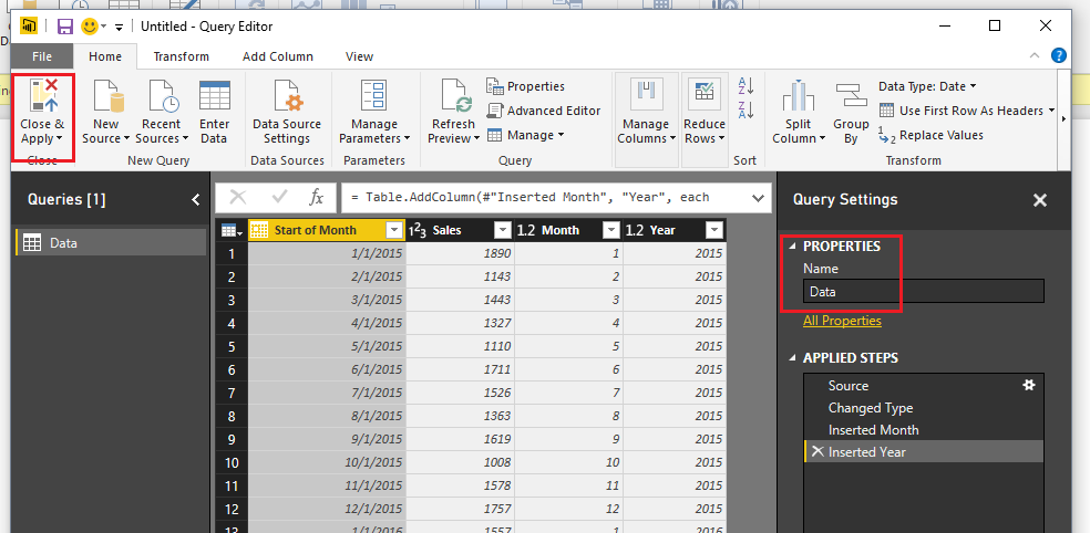
    let’s begin with loading our data and data transformations.  Open up PowerBI Desktop, Click the Get Data button on the Home ribbon and select Blank Query.  Click Connect to open the Query Editor.  Click Advanced Editor on the View ribbon.  While in the Advanced Editor paste the following code into the editor window, click Done to complete the data load.

    Note: If you need some more help loading the data follow this tutorial about loading data using the Advanced Query Editor.  This tutorial teaches you how to copy and paste M code into the Advanced Editor.

    let
     Source = Table.FromRows(Json.Document(Binary.Decompress(Binary.FromText("VdDBDcQwCETRXnyOFMAYcC1W+m9jV8BhfH1ygJ9zBr/8CvEaz+DYNL7nDAFjnWkTTNsUbIqnLfyWa56BOXOagy2xtMB5Vjs2mPFOYwIkikIsWd6IKb7qxH5o+bBNwIwIk622OCanTd2YXPNUMNnqFwomp0XvDTAPw+Q2uZL7QL+SC1Wv5Dpx/lO+Hw==", BinaryEncoding.Base64), Compression.Deflate)), let _t = ((type text) meta [Serialized.Text = true]) in type table [#"Start of Month" = _t, Sales = _t]),
     #"Changed Type" = Table.TransformColumnTypes(Source,{{"Start of Month", type date}, {"Sales", Int64.Type}}),
     #"Inserted Month" = Table.AddColumn(#"Changed Type", "Month", each Date.Month([Start of Month]), type number),
     #"Inserted Year" = Table.AddColumn(#"Inserted Month", "Year", each Date.Year([Start of Month]), type number)
    in
     #"Inserted Year"

    While still in the Query Editor rename the query to Data.  Then click Close & Apply to complete the data load into the data model.

    Load Monthly Data
    Load Monthly Data

    Next, make four measures.  On the Home ribbon click the New Measure button.  Enter the following to establish a reference date to the subsequent equations:

    Date Reference = DATE(2016,12,31)

    Enter in the following equation to calculate the last year monthly sales amount.

    LastYear = 
      VAR 
        CurrentDate = [Date Reference]
      RETURN
        CALCULATE( 
         SUM(Data[Sales]), 
         Data[Year] = YEAR(CurrentDate)-1
        )

    Note: Using the NOW() function calls the current time when the query was last run.  Thus, if you refresh your data next month the NOW() function wrapped in a YEAR() will return the current year from the date-time observed by PowerBI.

    Following the same process enter the following additional measures.  The ThisYear measure calculates the sales for the current month.

    ThisYear = 
      VAR 
       CurrentDate = [Date Reference] 
      RETURN
       CALCULATE(SUM(Data[Sales]),Data[Year] = YEAR(CurrentDate))

    Finally, add the calculation for the Year to Year comparison.

    YoY Percent Change = DIVIDE([ThisYear], [LastYear], 0)-1

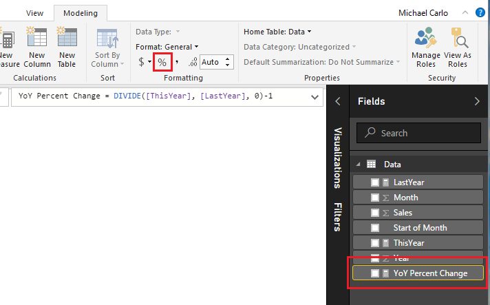
    Since the YoY Percent Change is a real percentage we need to change the formatting to a percent.  Click on the YoY Percent Change measure then on the Modeling ribbon click the symbol in the formatting section of the ribbon.

    Change Measure Format
    Change Measure Format

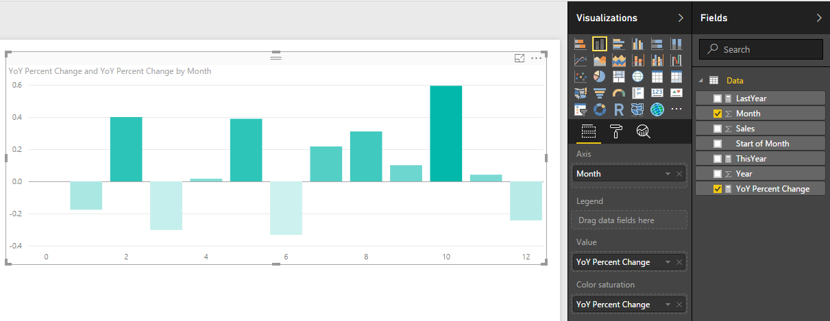
    Next, add a Stacked Column Chart with the following columns selected.

    Add Stacked Column Chart
    Add Stacked Column Chart

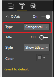
    OK, we have a chart, but it is kinda awkward looking right now.  The x-axis is the month number but we don’t have a month 0.  That simply does not make sense.  Let’s change some of the chart properties.  While having the Stacked Column Chart selected click on the Paint Roller in the Visualizations pane.  First, click on the X-Axis and change the Type to Categorical.

    Change X-Axis
    Change X-Axis

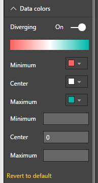
    Then click on the Data Colors and turn on Diverging.  Change the Minimum color to Red and the Maximum color to Green.  Set the Center to a value of 0.

    Change Colors
    Change Colors

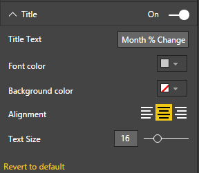
    Click on the Title change it something meaningful, Center the text and increase the font size.

    Change Title
    Change Title

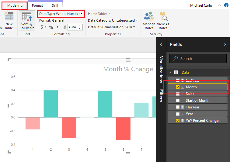
    Our bar chart looks much better.  However, the month numbers do not look quite right.  Visually the month indicators would be cleaner if we didn’t have any decimals.  Click on the Month field and then on the Modeling ribbon change the Data Type to Whole Number.  There will be a warning letting you know that you are changing the Data Type of the Whole number.  Click OK to proceed with the change.

    Change Month to Whole Number
    Change Month to Whole Number

    Another successful percent change tutorial completed.  I hope you enjoyed this year over year month comparison example.  Make sure you share if you like what you see.

  • Pareto Charting in PowerBI

    Pareto Charting in PowerBI

    The Pareto chart is a handy visual, but is not so easy to build in either excel or PowerBI.  In a Pareto chart, information is provided about an individual product or category as a bar, and a cumulative scale as a line which compairs all bars.  This type of visual can be extremely helpful when conducting failure mode analysis, causes of a problem, or even product portfolio balances.  For some more information on Pareto charts you can learn more here or here.  If you’re interested in building a Pareto chart in excel, I have found this post from Excel Easy to be helpful.

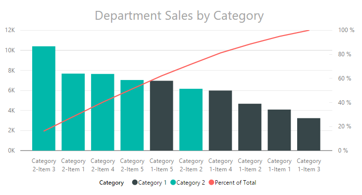
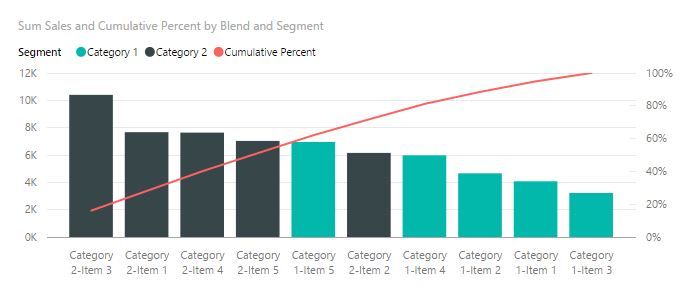
    To give you a little teaser of what we will be building today, below you will see an image of the final Pareto chart.  On the left side we have sales of units, and on the right is the cumulative percent of all sales.  Using the Pareto chart a user has the ability to see which products comprise the majority of your sales.  For example, the first 4 bars total approximately 50% of all sales.

    Pareto Final Product
    Pareto Final Product

    Alright, let’s get started.

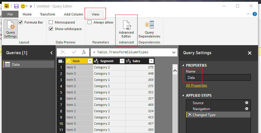
    Open up PowerBI Desktop, Click the Get Data button on the Home ribbon and select Blank Query.  Click Connect to open the Query Editor.  Click Advanced Editor on the View ribbon.  While in the Advanced Editor paste the following code into the editor window.

    Note: If you need some more help loading the data follow this tutorial about loading data using the Advanced Query Editor.  This tutorial teaches you how to copy and paste M code into the Advanced Editor.

    let
     Source = Excel.Workbook(Web.Contents("https://powerbitips03.blob.core.windows.net/blobpowerbitips03/wp-content/uploads/2016/10/Sample-Data.xlsx"), null, true),
     Table1_Table = Source{[Item="Table1",Kind="Table"]}[Data],
     #"Changed Type" = Table.TransformColumnTypes(Table1_Table,{{"Item", type text}, {"Sales", Int64.Type}, {"Segment", type text}})
    in
     #"Changed Type"

    Rename the Query to Data.  Once you’ve completed the data load your data should look like the following.

    Load Data to Query Editor
    Load Data to Query Editor

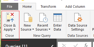
    On the Home ribbon click Close & Apply to complete the data load.

    Close and Apply
    Close and Apply

    Let’s begin with a little exploration of our data.

    Pro Tip: When I am building reports I often load the data and then immediately start building a couple of tables and slicers.  It helps me understand how my data reacts to the slicers and helps me determine how to shape the data so that the visuals will work properly.  For this example, we only have one table, but when loading data things can get rather complex due to loading multiple tables with multiple relationships.

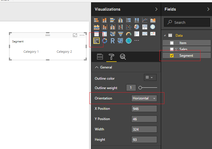
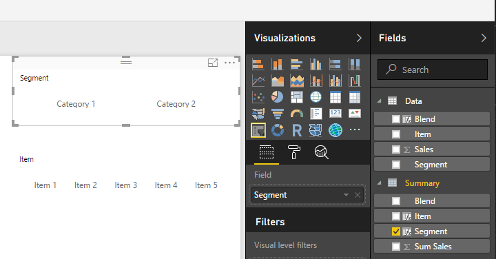
    Add a Slicer for the Segment.  Enhance the look of the slicer by changing it from a vertical to a horizontal slicer.  While the slicer is highlighted, click the Paint Roller expand the General section and change the orientation from vertical to Horizontal.

    Segment Slicer
    Segment Slicer

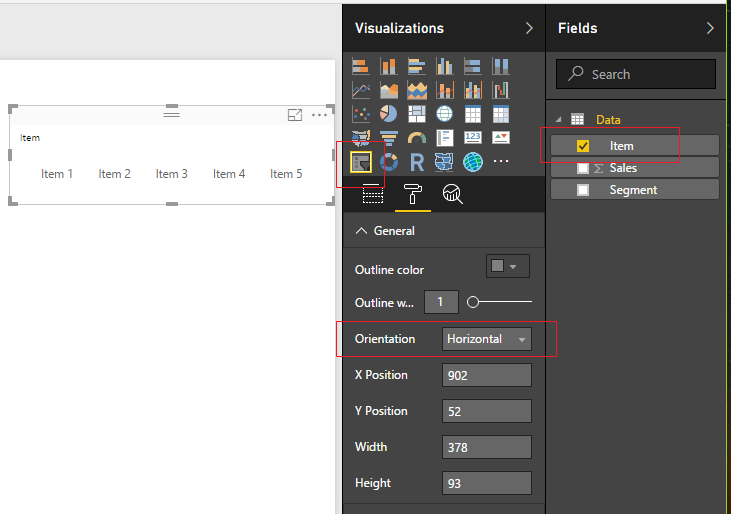
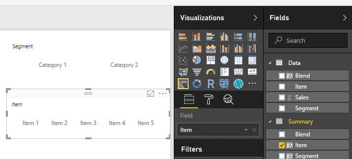
    Repeat the same process to add a Slicer for the item field.

    Item Slicer
    Item Slicer

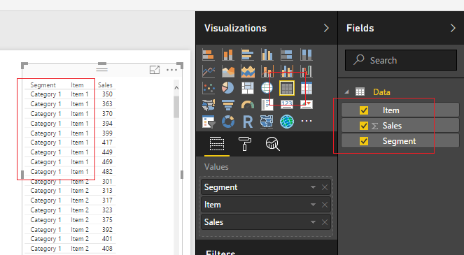
    Next, add a table view of all the fields.  Start with Segment, then Item and finally add Sales to the Table Visual.

    Data Table
    Data Table

    Notice, now that we added all the Fields, there are a number of repeating values.  We have Category 1 and Item 1 repeated 9 times.  In some cases, it will be necessary to have this level of data brought into the data model within PowerBI.  A common reason is that this level of granularity is required for other report pages, or visuals.  It is OK to bring large amounts of data, but as a method of best practice it is recommended that you bring in the data required to support the visuals.

    Now, to address these multiple items that we see in our data.  In the sample Pareto image provided at the beginning of this Tutorial we only had one bar for Category 2 Item 3.  Thus, we need to summarize each grouping of every Category and Item combination.  To do this we will construct a summary table.

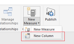
    First, we will create a unique Key that will be used to summarize each combination of Category and Item pair.  Click the bottom half of the New Measure button located on the Home ribbon.

    Calculated Column
    Calculated Column

    Enter the following DAX expression.  This new column titled Blend will be the unique Key that is utilized to summarize the data.
    Blend = Data[Segment]  &  "-"  &  Data[Item]

    Select the Modeling ribbon and then click on the New Table button.  Enter the following DAX expression.
    Summary = SUMMARIZE('Data', Data[Blend], "Sum Sales", SUM(Data[Sales]) )

    For more information on the SUMMARIZE function you can visit the Mircosoft Summarize documentation page.  In this equation we first select the table and in this case it is ‘Data’.  Then the column we want to summarize or group by is the Segment column noted as Data[Blend].  The next field is the title of the summarized field column, noted as “Sum Sales”.  Then DAX function that calculates the Sum of the column labeled Data[Sales], noted as SUM(Data[Sales]).  It is relevant to point out here that the SUMMARIZE function will only work with building a new table and not as a calculated column or measure.

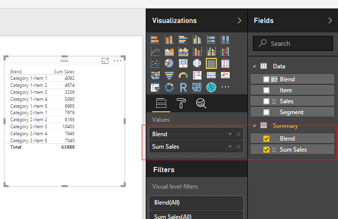
    Add a new Table visual to the report and include the two newly created fields from the Summary table.

    Summary Table Visual
    Summary Table Visual

    We have a field titled Blend which is our Key for all the summarized groupings.  Next, we will want to parse out the Segments and Items from this blend column.  We will want to use Category 1 & 2 in a slicer and the same for Items 1 to 5.  Highlight the summary table by clicking the grey space next to the word Summary.  Click the New Column button on the Modeling ribbon and enter the following DAX expression.
    Segment = PATHITEM(
       SUBSTITUTE(Summary[Blend], "-" , "|" ),
       1 )

    In this expression the Substitute function replaced the dash “-” with a “|” character.  Then the PATHITEM function can then parse the text into segments.  By entering a 1 we select the first item in the sequence.  For our example we only have two items, but when you’re working with file paths you can have multiple items in the path such as “\users\mike\my documents\my folder\”, which would equate to users = position 1, mike = position 2, my documents = position 3, etc..

    Add another new column with the following DAX expression for the item column.
    Item = PATHITEM( 
      SUBSTITUTE(Summary[Blend], "-" , "|" ),
      2 )

    Note: We changed the PATHITEM position from 1 to 2.
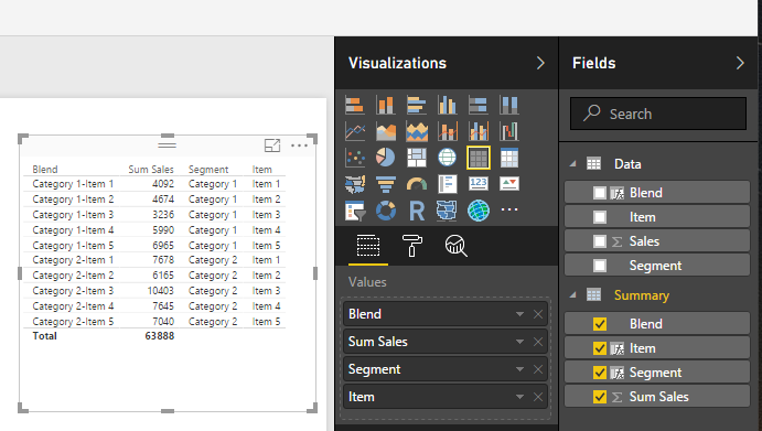
    Next add the newly created Segment and Item columns to our summary table visual that we created earlier.

    Add New Fields
    Add New Fields

    Nice job so far.  Now we have to modify our slicers to point to the new Item and Segment fields we created in the Summary table.  Select the Segment Slicer Visual and add the Segment Field from the Summary table.

    Update Segment Slicer
    Update Segment Slicer

    Update Item Slicer
    Update Item Slicer

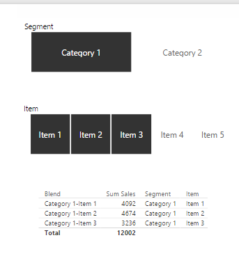
    Now that we have updated the slicers, we can now can control the table visual made from the Summary table.

    Select Category 1 and Items 1 to 3
    Select Category 1 and Items 1 to 3

    Pro Tip: To select multiple items in a slicer you can hold down the Ctrl button on the key board and click multiple slicer items.  This is how I was able to select Items 1 to 3.

    Now we are ready to build the measures that will support the Pareto chart.  Click on the bottom half of the New Measure button on the Home ribbon and select New Column.  Add the following DAX expression to rank all the items in the Summary table.

    Ranking = RANKX(  'Summary',   'Summary'[Sum Sales])

    Add a measure for the Cumulative total according to the new ranking column we created.  Click the top half of the New Measure button on the Home ribbon.  Add the following DAX expression.

    Cumulative Total = CALCULATE(
        SUM( Summary[Sum Sales] ),
        FILTER( ALLSELECTED( Summary ),
            Summary[Ranking] <= MAX( Summary[Ranking] )
        ))

    Repeat the add measure process and add a Total measure which will total only the items from the summary table that have been selected in the report view.  Add the following DAX expression.

    Total Sales = CALCULATE(
     SUM( Summary[Sum Sales] ) ,
     ALLSELECTED( Summary )
     )

    For the last measure, repeat the process to add another measure.  Enter the following DAX expression as a measure.

    Cumulative Percent = [Cumulative Total] / [Total Sales]

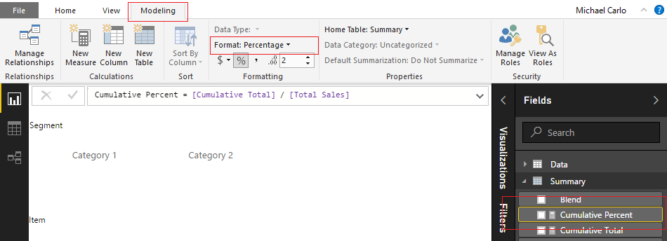
    The Cumulative Percent measure is a calculated as a percentage, thus we need to change this measure’s formatting to percentage.  Click the measure labeled Cumulative Percent then change the Format to Percentage which is found on the Modeling ribbon.

    Change Formatting
    Change Formatting

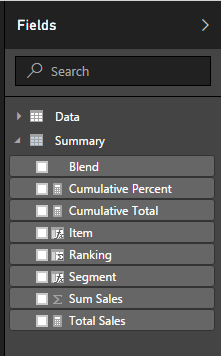
    Your Summary table should now look like the following.

    Updated Fields List
    Updated Fields List

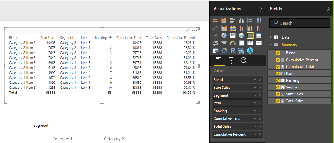
    To see all the calculations that we just created add all the fields from the Summary table to the Summary table visual we created earlier.

    Full Summary Table Visual
    Full Summary Table Visual

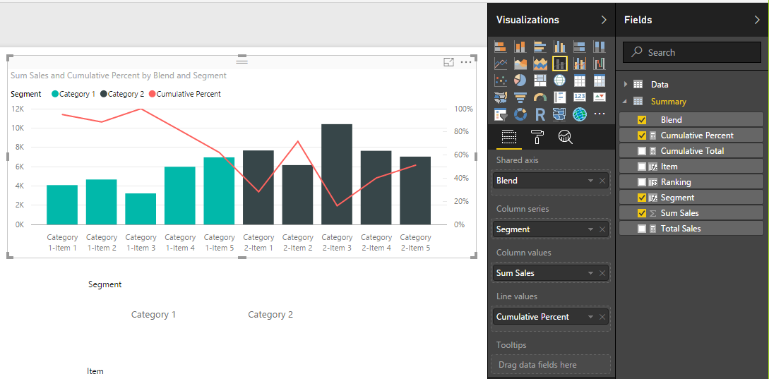
    At last, we are ready to add the Pareto chart.  Add the following fields to the line and stacked column chart.

    Add Line and Stacked Bar Chart
    Add Line and Stacked Bar Chart

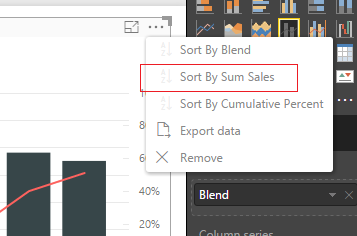
    Order the data in descending order by the number of sales by click the visual’s Ellipsis and selecting Sort By Sum Sales.

    Sort by Sales
    Sort by Sales

    This changes the order of the items to make a Pareto chart.

    Final Pareto Chart
    Final Pareto Chart

    Thanks for following along.  Share if you enjoyed this tutorial.

  • Map with Data Labels in R

    Map with Data Labels in R

    Mapping is one of the better features of PowerBI.  It is one of the more distinguishing feature differences between Excel and PowerBI.  You can produce a map inside an excel document using Bing maps, however, the experience has always felt a little like an after-thought.  Mapping within PowerBI has a planned, and thoughtful integration.  While the mapping functionalities within PowerBI Desktop are far improved when compared to excel, there are still some limitations to the mapping visuals.  This past week I encountered such an example.  We wanted to draw a map of the United States, add state name labels and some dimensional property like year over year percent change.

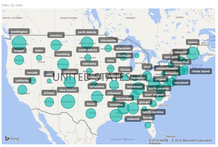
    I started with the standard map visual, but this didn’t work because there is no ability to shade each state individually.  This just looked like a bubbled mess.

    Globe Map Visual
    Globe Map Visual

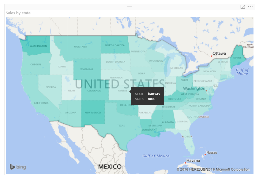
    Next, I tried the Filled Map visual.  While this mapping visual provides the colored states it lacks the ability to add data labels onto the map.  Clicking on the map would filter down to the selected state, which could show a numerical value.  Alternatively, you can place your mouse over a state and the resulting tag will show the details of the state (hovering example provided below).

    Filled Map Visual
    Filled Map Visual

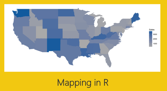
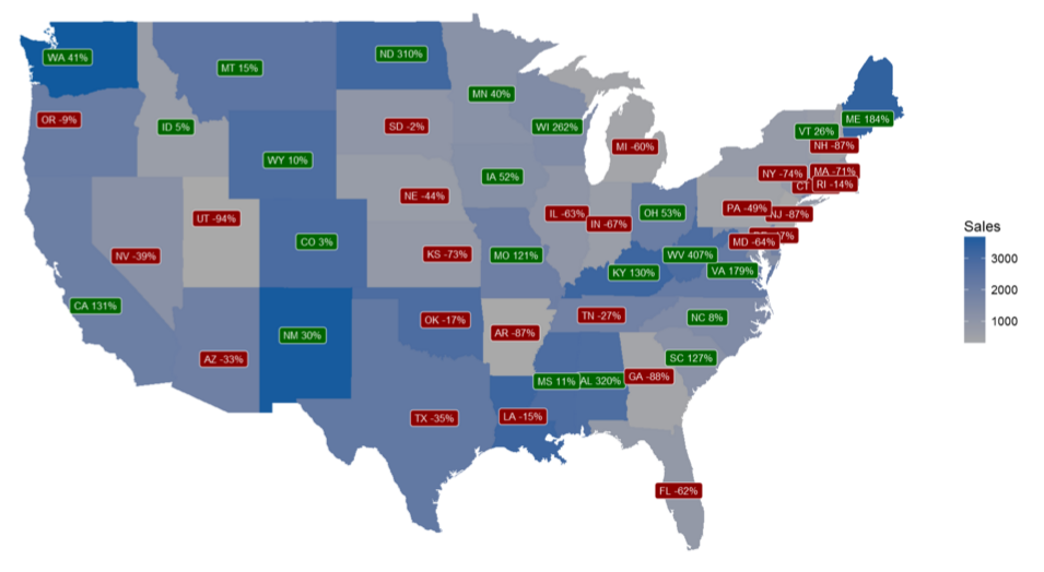
    Still this did not quite meet my visual requirements.  I finally decided to build the visual in R which provided the correct amount of flexibility. See below for final result.  You can download the pbix file from the Microsoft R Script Showcase.

    R Map Visual
    R Map Visual

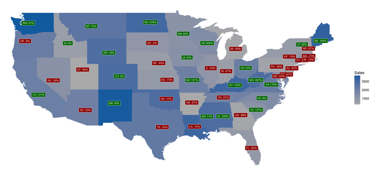
    In this visual, each state is shaded with a gradient color scale.  The states with the lowest sales are grey and the states with higher sales numbers transition to dark blue.  The darker the blue the more sales the state saw.  Each state has an applied label.  The color of the label denotes the percent change in sales.  If the color is green then the sales this year were higher than last year, red means that the state sales were lower this year.  The state name is listed in the label as well as the calculation for the year over year percent change.

    Alright, let’s start the tutorial.

    First, before we open PowerBI we need to load the appropriate packages for R.  For this visual you will need to load both the maps and the ggplot2 packages from Microsoft R Open.

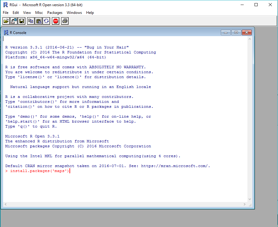
    Open the R console and use the following code to install maps.

    install.packages('maps')

    Install Maps Package
    Install Maps Package

    Repeat this process for installing ggplot2.

    install.packages('ggplot2')

    After installing the R packages we are ready to work in PowerBI Desktop.  First, we need to load our sample data.  Open up PowerBI Desktop and start a blank query.  On the View ribbon in the query editor open the Advanced Editor and enter the following M code.

    Note: If you need some more help loading the data follow this tutorial about loading data using the Advanced Query Editor.  This tutorial teaches you how to copy and paste M code into the Advanced Editor.

    let
      Source = Excel.Workbook(Web.Contents("https://powerbitips03.blob.core.windows.net/blobpowerbitips03/wp-content/uploads/2016/10/State-Data.xlsx"), null, true),
      StateData_Table = Source{[Item="StateData",Kind="Table"]}[Data],
      #"Changed Type" = Table.TransformColumnTypes(StateData_Table,{{"StateName", type text}, {"Abb", type text}, {"TY Sales", Int64.Type}, {"state", type text}, {"Latitude", type number}, {"Longitude", type number}, {"LY Sales", Int64.Type}, {"Chng", type number}}),
      #"Renamed Columns" = Table.RenameColumns(#"Changed Type",{{"TY Sales", "Sales"}})
    in
      #"Renamed Columns"

    After pasting the code into the Advanced Editor click Done to load the data.  While in the Query Editor, rename the query to be StateData, then click Close & Apply on the Home ribbon.

    Load Mapping Data
    Load Mapping Data

    We still need to prepare the data further by adding two calculated columns.  Click the bottom half of the New Measure button on the Home ribbon and select New Column.

    Add New Column
    Add New Column

    Enter the following code into the formula bar that appears after clicking New Column.

    Change = StateData[Abb] & " " & ROUND(100*StateData[Chng],0) & "%"

    Change Column Measure
    Change Column Measure

    Again, click on the New Column button found on the Home ribbon and add the code for a color column.

    Color = if(StateData[Chng] > 0 , "Dark Green", "Dark Red")

    Color Column Measure
    Color Column Measure

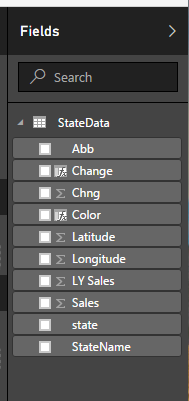
    The Fields list should now look like the following.

    Fields List
    Fields List

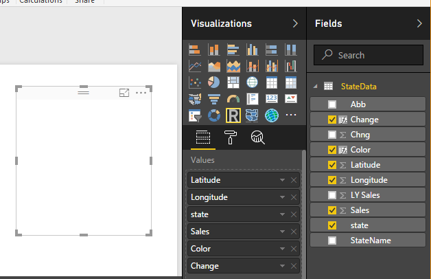
    Add the R visual with the following fields.

    R Visual Fields
    R Visual Fields

    Add the following R script into the R Script Editor.

    # Load the ggplot2 and maps packages
     library(ggplot2)
     library(maps)
    
    # Load the mapping data into a dataframe called states_map
     states_map <- map_data("state")
    
    # Start ggplot2 by sending it the dataset and setting the map_id variable to state
     ggplot(dataset, aes(map_id = state)) +
    
    # Add the map layer, define the map as our data frame defined earlier
     # as states_map, and define the fill for those states as the Sales data
     geom_map(map = states_map, aes(fill=Sales)) +
    
    # Add the data for the labels
     # the aes defines the x and y cordinates for longitude and latitude
     # colour = white defines the text color of the labels
     # fill = dataset$Color defines the label color according to the column labeled Color
     # label = dataset$Change defines the text wording of the label
     # size = 3 defines the size of the label text
     geom_label( aes(x=Longitude, y=Latitude), 
      colour="white", 
      fill=dataset$Color, 
      label=dataset$Change, size=3
      ) +
    
    # define the x and y limits for the map
     expand_limits(x = states_map$long, y = states_map$lat) +
    
    # define the color gradient for the state images
     scale_fill_gradient( low = "dark grey", high = "#115a9e") +
    
    # remove all x and y axis labels
     labs(x=NULL, y=NULL) +
    
    # remove all grid lines
     theme_classic() +
    
    # remove other elements of the graph
     theme(
      panel.border = element_blank(),
      panel.background = element_blank(),
      axis.ticks = element_blank(),
      axis.text = element_blank()
      )

    After adding the R script press the execute button to reveal the map.

    Paste R Script
    Paste R Script

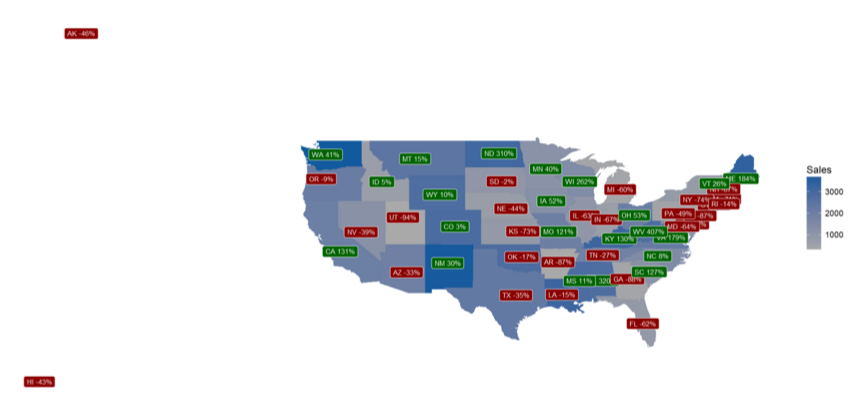
    Final Map Product
    Final Map Product

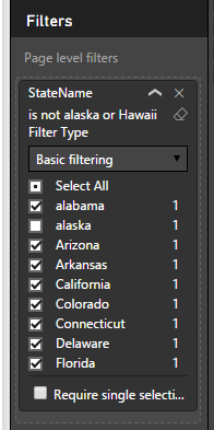
    Notice how we have data included for Alaska and Hawaii but those states are not drawn.  We want to remove the Alaska and Hawaii data points.  Add the StateName field to the Page Level Filters and then click Select All.  Now, un-check the boxes next to Alaska and Hawaii.  The data is now clean and the map correctly displays only the continental United States.

    Page Level Filters
    Page Level Filters

    Here is the filtered final map product.

    Filtered Final Map
    Filtered Final Map

    Thanks for following along.  I hope you enjoyed this tutorial.  Please share if you liked this content.  See you next week.